Simulation Interactions Diagram Panel
Display information on protein-ligand interactions derived from a simulation, in graphical form. The diagrams show RMSD and RMSF measures for proteins, including backbone, side-chain, and secondary structure changes; ligands, including internal and external motions; and protein-ligand contacts, including H-bonds, hydrophobic, ionic, and water-bridge contacts.
To open this panel: click the Tasks button and browse to Classical Simulation → Simulation Interactions Diagram.
- Using
- Features
- Additional Resources
Using the Simulation Interactions Diagram Panel
The purpose of this panel is to display graphically information about the behavior and interactions of proteins and ligands during the course of a simulation. For example, you can examine to what extent a hydrogen bond between a ligand and a protein residue is maintained during the simulation, whether the ligand moves in and out of the binding site, what are the more rigid regions of the protein and what are the flexible regions, how well is a water bridge maintained, how flexible the ligand is in the binding site. This information could be used to validate a ligand pose, or propose modifications to the ligand or to the protein.
To generate the analysis data, you can click the Load button and select an output -out.cms file that has an associated trajectory, and run the analysis. Once the analysis is run, you can load the event analysis file (.eaf) and examine the various graphical representations of the RMSD, RMSF, contacts, and torsions.
You can create a PDF file that contains all the charts in the panel, along with explanatory text, or you can export just the charts as images. You can also export the data to a plain text file if you want to do your own analyses or processing of the data.
Simulation Interactions Diagram Panel Features
- Load button
-
Load the results of an analysis of the simulation interactions, from an event analysis file (
.eaf), or load a simulation that has a trajectory (-out.cmsfile) and run the analysis. When you load a simulation, the SID Analysis Setup dialog box opens, in which you can specify ASL expressions that define the protein and the ligand, and select the analysis types that you want to run. Clicking Run in the dialog box runs the analysis on the trajectory and loads the results. The-out.cmsfile is imported into Maestro as well, when you load the chosen file. - Generate Report button
-
Generate output that contains the information in the panel in one or more formats:
- PDF—Generate a PDF file that contains the diagrams with explanatory text.
- Plots—Save all the diagrams in the panel in PNG or SVG format.
- Data—Export the data used to generate the diagrams as plain text files.
- Tabs
-
Smooth the plots by averaging over the chosen number of residues.
- Diagram
-
The plots of the RMSF as a function of simulation time and other markers are displayed in this area. The legend for the various RMSF values is given at the top. When you move the pointer over the plot area, a vertical line is displayed at the residue position. The chain, residue number and name are displayed to the left of the line, and the RMSF values are displayed to the right of the line.
L-RMSF tab
This tab displays root-mean-square fluctuations (RMSF) for each atom in the ligand chain. The RMSF for the atoms is the time-averaged fluctuation of the square deviation of the ligand heavy atoms over the entire simulation time, after superposition on the reference frame.
- Show ligand RMSF options
-
Choose an option to display the RMSF for a given alignment of the ligand. Alignment on the ligand represents internal fluctuations of the ligand; alignment on the protein represents fluctuations with respect to the binding site.
- Ligand structure
-
The 2D structure of the ligand is shown in this panel, colored by element, and without hydrogens shown. The atom index used in the plot can be shown on the figure by selecting Atom numbers. The atom at the cursor position in the plot is highlighted with a blue square.
- Atom numbers option
-
Select this option to show the atom numbers in the ligand structure.
- Diagram
-
The plots of the RMSF as a function of simulation time are displayed in this area. The legend for the various RMSF values is given at the top. When you move the pointer over the plot area, a vertical line is displayed at the atom position. The atom number, PDB name and atom type are displayed to the left of the line, and the RMSF values are displayed to the right of the line.
PL-Contacts tab
This tab displays information on protein-ligand contacts. A bar chart gives the fraction of the simulation time that the ligand is in contact with protein residues, and another chart shows the contacts as a function of simulation time.
- Contact options
- Average contacts bar chart
- Trajectory range section
- Legend
- Histogram information section
- Contacts diagram
- Contact options
-
Select these options to display different types of contacts. If you select a single option, the chart shows a breakdown of the contact type into more specific interactions:
- H-bonds—Show hydrogen bonds to the protein, broken down into backbone and side chain, donor and acceptor. Hydrogen bonds are defined by distances and angles of the D-H...A-X atom arrangement: a H-A distance less than 2.8Å, a D-H-A angle greater than 120°, and a H-A-X angle greater than 90°.
- Hydrophobic
- pi-pi stacking—two aromatic groups stacked face-to-face, with distance between centroids less than 4.4Å and angle between planes less than 30°, or face-to-edge, with distance between centroids less than 5.5Å and angle between planes greater than 60°.
- pi-cation—aromatic and charged group centroids within 4.5Å, and
- general—hydrophobic side chain within 3.6Å of ligand aromatic or aliphatic carbon.
- Ionic—Show interactions between oppositely charged atoms on the ligand and the protein that are within 3.7Å.
- Water bridge—Show interactions that involve hydrogen bonding via a water bridge molecule, broken down into protein donor and protein acceptor. The geometric criteria are a H-A distance less than 2.7Å, a D-H-A angle greater than 110°, and a H-A-X angle greater than 80° for the hydrogen bonds to the bridging water.
- Halogen bonds—Shows halogen bonds to the protein.
If you select multiple options, the sums of the specific interactions are displayed.
- Average contacts bar chart
-
This diagram shows a bar chart of the average number of interactions over the simulation time. The number can be greater than one if the protein makes more than one contact of a particular type with the ligand, e.g. two hydrogen bonds to the same ligand atom.
If multiple interaction types are selected, the bar chart shows the total for each type. If a single interaction type is selected, the bar chart shows the breakdown for the specific subtypes.
When you move the pointer into a bar segment, information for that bar segment is shown in the Information section, to the right.
- Trajectory range section
-
This area shows the range of the trajectory that is selected for analysis. You can change the range by clicking Set Range and setting the lower and upper frame numbers in the dialog box that opens.
- Legend
-
The legend shows the color coding for the selected interaction types or subtypes.
- Histogram information section
-
The information section shows the average number of contacts and the number of frames that have the contact for the bar segment in the chart over which the pointer is resting.
- Contacts diagram
-
This diagram shows the number of interactions as a function of time for each residue. The top chart shows the total number of the selected interactions as a function of time. The bottom chart shows the number of interactions for each residue in contact with the ligand as a function of time. This number is an integer, and the number is color-coded in shades of orange. When you hover the pointer over the bottom chart, a pop-up containing information on the specific residue and frame data appears.
LP-Contacts tab
This tab shows a schematic diagram of ligand-protein interactions.
- Min contact strength slider
-
Use this slider to set the contact strength (average interaction) for which protein residues are displayed.
- Trajectory range section
-
This area shows the range of the trajectory that is selected for analysis. You can change the range by clicking Set Range and setting the lower and upper frame numbers in the dialog box that opens.
- Ligand interaction diagram
-
This area shows the 2D structure of the ligand and the protein residues it interacts with. The diagram features are explained in the legend below. The interaction strengths are indicated on the diagram.
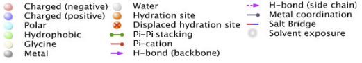
- Legend
-
Shows the list of features that can appear in the diagram and what they represent.
L-Torsions tab
This tab shows charts of the torsional conformation of each rotatable bond in the ligand. Up to 10 charts are displayed. If there are more than 10 rotatable bonds, you can step through the sets of 10 charts (or bonds).
- Polar plots and bar charts
- Trajectory range section
- Ligand structure
- Previous and Next buttons
- Legend button
- Polar plots and bar charts
-
The polar plots show the conformation of the ligand as a function of time, where the radial coordinate is the simulation time, and the angular coordinate the torsional angle. The bar charts show the probability of the torsions as a function of angle. They represent the average over the simulation time. If the torsional potential information is available, this is plotted on the bar charts. The color of the plot matches the color coding of the rotatable bond on the ligand structure. The ligand strain is displayed under the X axis when the torsion potential is nonzero.
These plots give information on the conformational stability of the ligand, and with the torsional potential, give information on possible ligand strain in the protein-bound conformation.
- Trajectory range section
-
This area shows the range of the trajectory that is selected for analysis. You can change the range by clicking Set Range and setting the lower and upper frame numbers in the dialog box that opens.
- Ligand structure
-
This area shows the structure of the ligand, with the rotatable bonds marked with distinct colors. Only 10 bonds at a time are marked.
- Previous and Next buttons
-
If there are more than 10 rotatable bonds, these buttons are activated, so that you can step through sets of 10 rotatable bonds.
- Legend button
-
Opens a panel that explains the polar plots and bar charts.
L-Properties tab
This tab shows plots and bar charts of six ligand properties: polar surface area (PSA), solvent-accessible surface area (SASA), molecular surface area (MolSA), intramolecular hydrogen bonds (intraHB), radius of gyration (rGyr), and ligand RMSD with respect to the initial conformation (the same as in the PL-RMSD tab). For each property there is a chart that shows the value of the property as a function of time; to the right there is a bar chart that shows the proportion of time spent in each of 10 value ranges, divided equally over the range of property values.
- Trajectory range section
-
This area shows the range of the trajectory that is selected for analysis. You can change the range by clicking Set Range and setting the lower and upper frame numbers in the dialog box that opens.
- Plots and bar charts
-
The plots of the ligand properties as a function of simulation time are displayed in this area. When you move the pointer over the plot area, a vertical line is displayed in all plots. The simulation time is displayed to the left of the line, and the property value is displayed to the right of the line, in each plot.