Timings for Typical Jaguar Jobs
Employing quantum mechanics software for practical use depends on managing the computational and financial cost incurred by the calculations, which can be significant in many cases. To understand these costs for Jaguar, timings for typical property calculations using common theoretical methods are visualized in several plots below (Figures 1-7).
Parallel to this effort, the Jaguar Timer tool has been developed to allow estimates of the overall wall time of a Jaguar job based upon (1) its input file and (2) the desired number of CPUs. These estimated wall times are derived from a machine learning model trained on a diverse set of calculations. Please refer to the Jaguar Timer documentation for more details.
It is important for users to be aware that the timings of their calculations may differ from either those plotted herein or those predicted by Jaguar Timer. The magnitude of these differences can depend on several different factors that are explained below.
Different methods within density functional theory (DFT) – such as e.g. hybrid, GGA, meta-GGA, range-corrected functionals – employ different implementations that can affect their general speed as well as their performance for a given system. See Figures 1-3 for various functional timings. Additionally shown in Figure 3 is the impact of basis set size, which can dramatically impact the calculation time. Properties incur different cost (Figure 4). Different job parameters can impact the time: usage of the pseudospectral approximation will speed up calculations (Figure 5), whereas employing different solvation models will add cost (Figure 6).
Both the quality of the initial guess structure and complexity of the corresponding electronic structure will greatly impact the wall times, since they impact both the number of SCF and geometry optimization cycles required to achieve the desired convergence. The number of cycles may also vary based on the quality of the method. Relatedly, for a given molecular size (e.g., weight, or the number of basis functions) different chemical moieties will impact the timings (see Figure 2). The diversity plotted below represents a tiny fraction of chemical space. For example, open-shell systems or flexible systems can often require more effort.
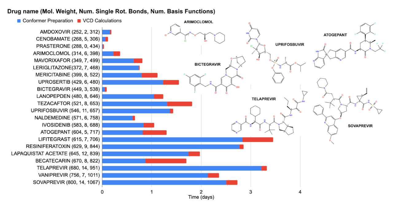
Making reasonable predictions for the property of a given system may only be possible by synthesizing calculations for a set of conformers of a given species. This approach can greatly increase the number of calculations and thus the overall time of a given prediction. Figure 7 shows this for VCD workflows calculations for several different molecules.
Lastly, timings may be greatly affected by the hardware and the number of CPUs requested. Unless otherwise stated, all calculations plotted herein were performed using the following:
- Jaguar from 23-1, build 128
- Default keyword settings
- Intel(R) Xeon CPU @ 2.80 GHz, x86_64 architecture
Figure 1. B3LYP-D3/6-31G** single-point energy timings for linear alkanes (CnH2n+2).
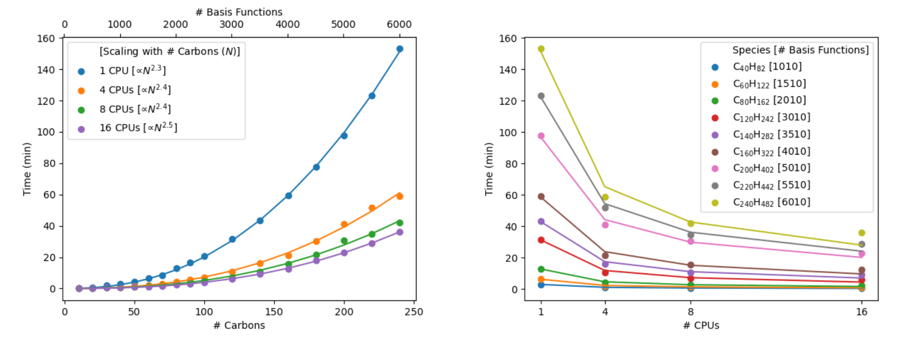
Figure 2. B3LYP-D3/6-31G** single-point energy timings for 45 OLED and 80 OPV molecules.
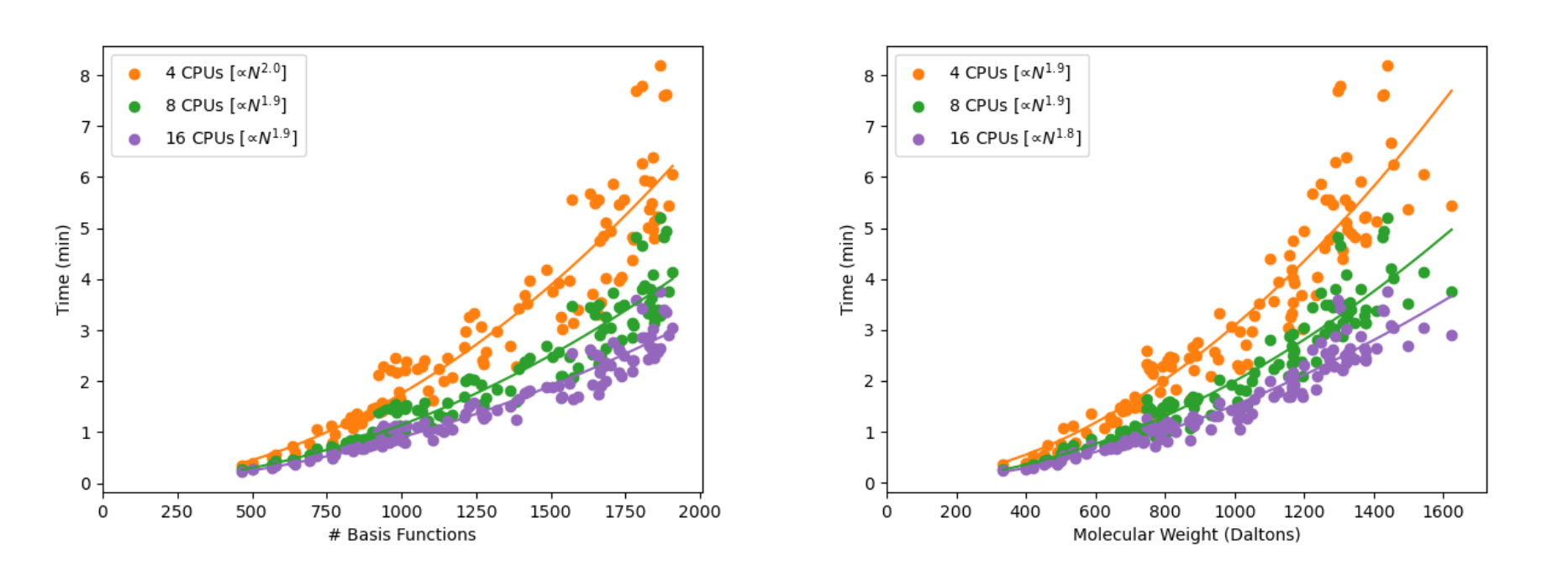
Figure 3. Single-point energy timings for different DFT functionals for linear alkanes (CnH2n+2): (left) 6-31G** and (right) def2-TZVP.
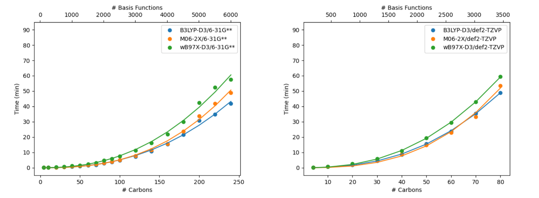
Figure 4. B3LYP-D3/6-31G** timings for linear alkanes (CnH2n+2) for various molecular properties: (top left) gradient, (top right) frequency, (middle left) TDDFT-TDA [5 lowest roots], (middle right) polarizability and hyperpolarizability, (bottom) NMR chemical shieldings.
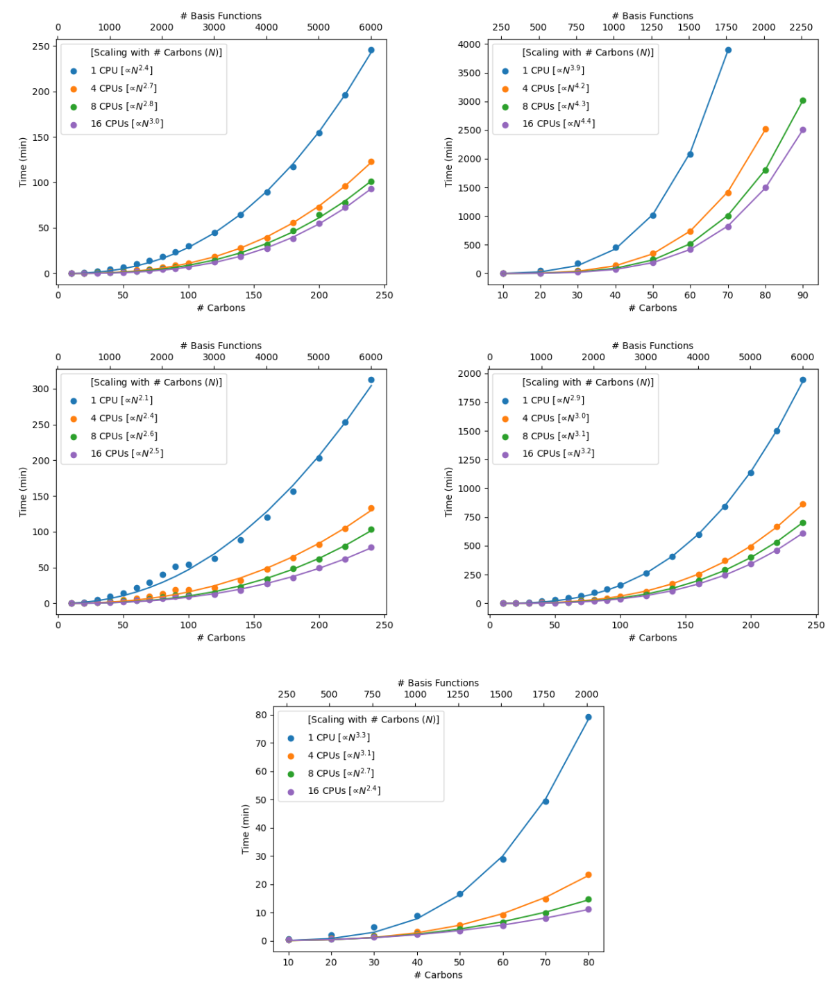
Figure 5. Cost differences for employing the pseudospectral approximation in single-point energy calculations of linear alkanes (CnH2n+2).
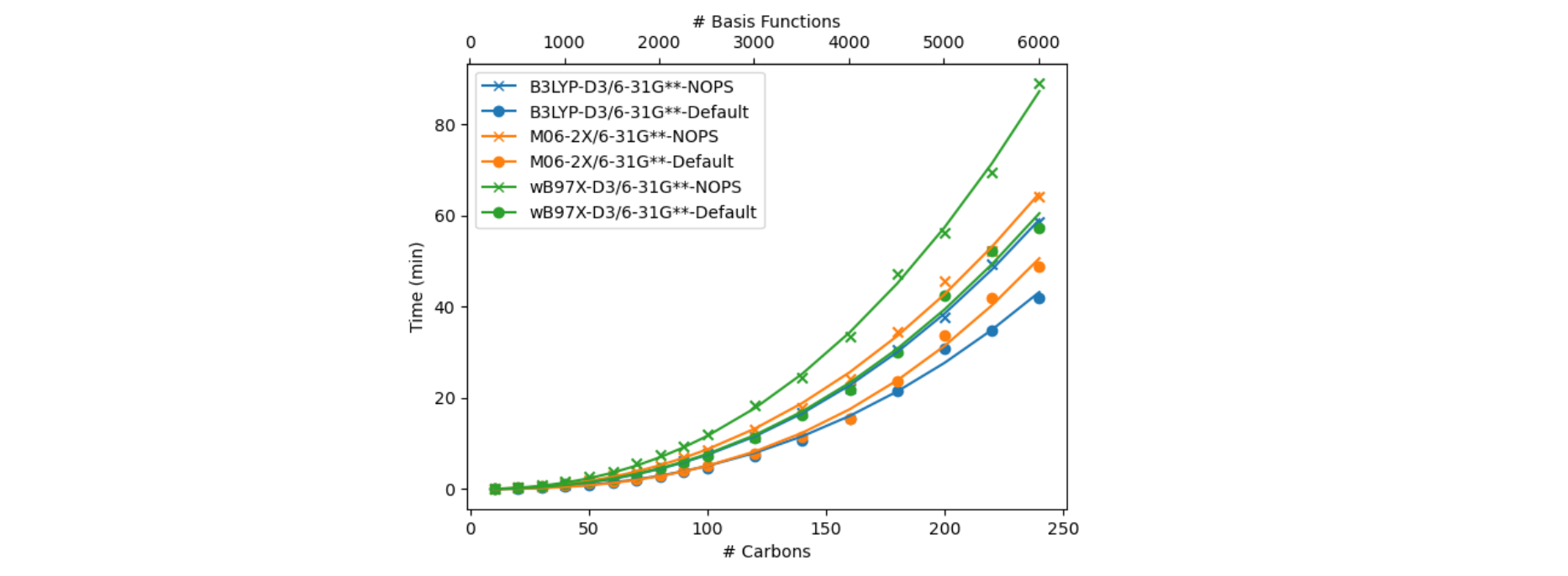
Figure 6. Cost differences when employing an implicit solvent model versus gas-phase for linear alkanes (CnH2n+2). The solvent model plotted here is a conductor-like polarizable continuum model (CPCM). Timings are compared both with and without (NOPS) the pseudospectral approximation, depicted on the left and right, respectively. Note that these calculations employ the default approach in Jaguar where both a gas-phase and solution-phase SCF calculation are done when CPCM energies are requested.
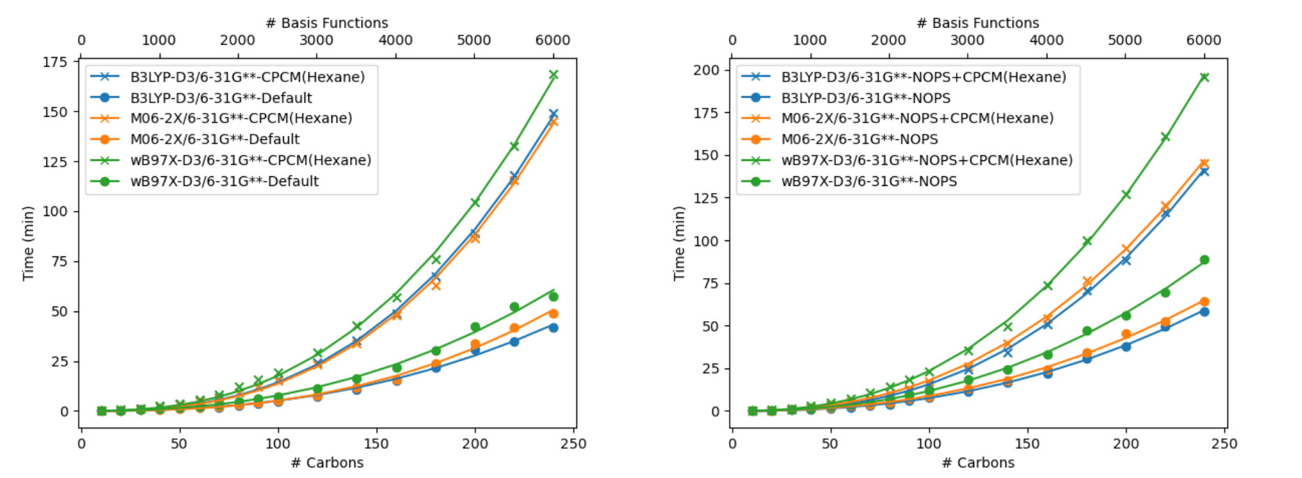
Figure 7. Timings for vibrational circular dichroism (VCD) workflow timings for drug-like molecules. For each workflow, we select conformers used to generate the spectrum by conformer sampling with a force field using Macromodel, which is filtered using DFT optimizations and DFT optimizations and frequency calculations. The individual VCD contributions of low-lying conformers are determined by Boltzmann averaging. Each calculation done with B3LYP-D3/LACVP** using 16 CPUs on a single compute node.