MxMD Custom Cosolvent Probes
To add custom probes to the MxMD workflow, first generate a pure cosolvent box, then simulate a water/cosolvent system to determine if the cosolvent is miscible with water.
Pyrazole is used as example in this topic.
Drawing a Cosolvent Molecule
Use the 2D Sketcher Panel to draw a two-dimensional representation of a single molecule of your custom cosolvent. Export the file as a Maestro file—e.g., pyrazole.mae. See Export Dialog Box for more information.
Generating a Cosolvent Probe System
The workflow will execute the following steps:
- Generate a cosolvent system with 343 molecules (73)
- Equilibrate pure cosolvent system (148 ps)
- Simulate pure cosolvent system, NPT ensemble, 300 K, 2 fs timestep (total: 20,000 ps)
- Add water to the cosolvent system in a 1:1 ratio (by weight)
- Equilibrate the cosolvent/water mixture (total: 6,300 ps)
- Simulate for the cosolvent/water mixture, NPT ensemble, 300 K, 2 fs timestep (total: 50,000 ps)
- Calculate radial distribution functions and generate plots.
Submit the workflow with the command:
$SCHRODINGER/utilities/multisim pyrazole.mae \
    -JOBNAME pyrazole -HOST GpuHost \
    -m $SCHRODINGER/mmshare-*/data/desmond/mxmd_cosolvent_probe_generation.msj
Replace GpuHost with an entry of the schrodinger.hosts file that has a GPU.
As a result of running this workflow, a PNG image is generated, displaying four radial distribution functions g(r) calculated between the center of masses of the molecules (Figure 1). The following radial distribution functions are reported:
- Probe – Neat: g(r) of probes in the pure cosolvent system
- Probe – with Water: g(r) of probes in cosolvent/water mixture
- Water – Neat: g(r) of water molecules in a pure water system
- Water – with Probe: g(r) of water molecules in cosolvent/water mixture
The radial distribution functions can be used to judge whether the cosolvent probe is miscible with water (e.g. pyrazole) or immiscible (e.g. oxolane) [3]. For miscible probes the radial distribution functions converge to 1.0 at large distances (e.g. 12 Å), indicating an even distribution of probes. For immiscible probes the radial distribution functions converge to numbers large than 1.0, indicating an uneven distribution of probes.
|
|
|
|
Miscible |
Immiscible |
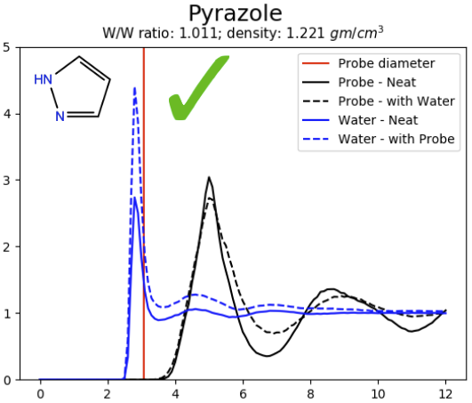
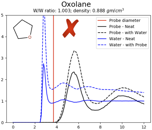
Figure 1: Radial distribution functions of pure cosolvent systems pyrazole (left) and oxolane (right).
Generating Custom Cosolvent Systems from Trajectories
If the custom cosolvent probe is miscible, generate the cosolvent simulation boxes by running the following command on the command line:
$SCHRODINGER/run generate_solvent_box.py pyrazole_probe-out.cms pyrazole -t pyrazole_probe.xtc -s "100:-1:10" -pdbres PZO
This command discards the first 100 frames, extracts 10 snapshots from the remaining trajectory and stores them in a file pyrazole.box.mae. Select a suitable PDB residue name, e.g., PZO for pyrazole.
Using Custom Probes
To use a custom probe in MxMD simulations, run the job from the command line with the -custom-probe-dir option to specify the directory that contains the MAE file with the cosolvent structures.