Residue Mutation Results

When a Residue Scanning or Antibody Humanization: Residue Mutation job finishes, the Residue Scanning Viewer, Affinity Maturation Viewer or Humanize Antibody Viewerpanel opens, displaying changes in properties for each mutation, and a graph of one of the properties against the row number.

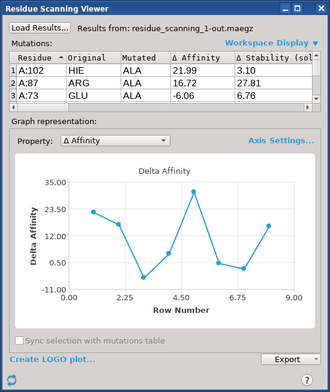
If you want to examine results from a job that was completed earlier, you can open this panel: to open it, click the Tasks button and browse to Biologics → MM-GBSA Residue Scanning Results . You can then click Load Results to locate the Maestro file (.maegz) that contains your results and import it into the current project. For information on using this panel, see MM-GBSA Residue Scanning/Humanize Antibody Viewer Panel.

The results are listed in the Mutations table, with one mutated structure per row. The mutations in each structure are identified by the residue positions and the original and mutated residue names. For residue scanning, there is only one mutation per structure, but for affinity maturation, there may be multiple mutations. The properties that were calculated for each mutant are listed in the table. The properties are described briefly in Table 1. Some of these properties are described in more detail below. In addition to the properties listed, the change in the Prime energy components for the stability and affinity properties are also available in the Project Table (see Table 1 in Prime Energy Properties for a description of the components). All properties are calculated after the refinement is performed, and so include relaxation of the protein after mutation.

For affinity maturation, residue-level properties are summed, so they represent total changes due to the mutations. Dividing by the number of residues would give the average change in these properties. The properties for the individual residues are not reported.

Binding Affinity Prediction Method

The change in the binding affinity of the protein due to the mutation is calculated from the two individual binding energies, which can be represented as follows:

R + L → R·L       ΔG(bind)

R + L' → R·L'       ΔG'(bind)

where R is the receptor, L is the ligand in the parent, and L' is the mutated ligand. R+L and R+L' represent the separated receptor and ligand. R·L and R·L' represent the receptor bound to the ligand. The change in binding affinity is

ΔΔG(bind) = ΔG'(bind) − ΔG(bind)

The calculations are done with Prime MM-GBSA, which uses an implicit (continuum) solvation model. A negative value indicates that the mutant binds better than the parent protein.

In addition to the binding affinity property, contributions to this property from the components of the Prime Energy are also calculated—see Prime Energy Properties for more information. The binding affinity and its contributions are given in energy units.

Stability Prediction Method

The stability of the protein due to the mutation is calculated from a thermodynamic cycle, which can be represented as follows:

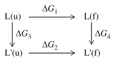
where L(u) is the unfolded parent protein, L(f) is the folded parent protein, L'(u) is the unfolded mutated protein, and L'(f) is the folded mutated protein. The change in stability is

ΔΔG(stability) = ΔG₂ − ΔG₁ = ΔG₄ − ΔG₃

Experiment measures ΔG₁ and ΔG₂, but the calculation of ΔΔG(stability) uses ΔG₃ and ΔG₄ with model unfolded proteins. The unfolded protein is represented as a tripeptide, A-X-B, where X is the residue that is mutated, and A and B are its neighbors, capped with ACE and NMA. The assumption is that the remaining interactions in the unfolded state are negligible. The calculations are done with Prime MM-GBSA, which uses an implicit (continuum) solvation model.

For a complex of two or more proteins, the change in stability due to the mutation is calculated with respect to the protein in the complex. The geometry used for the protein is that of the complex, so the calculated stability will depend on the complex. If you want the change in stability on mutation of just the protein (L), run the calculation for that protein in solvent, not in the complex. The change in stability of the protein in the complex is related to the change in stability of the protein in solvent by the addition of the change in binding affinity,

ΔΔG(stability,complex) = ΔΔG(stability, solvent) + ΔΔG(bind)

In addition to the stability property, contributions to this property from the components of the Prime Energy are also calculated—see Prime Energy Properties for more information. The stability property and its components are given in energy units.

Surface Complementarity Method

The surface complementarity is calculated using the method of Lawrence and Colman [10], which is outlined here. The complementarity at any point on the molecular surface (Connolly surface [11]) of one protein (A) is determined by finding the nearest point on the molecular surface of the other protein (B), and comparing the vectors normal to the two surfaces at those points, with a weighting function involving the distance between the points. Perfect complementarity is achieved if the vectors are parallel and the distance is zero. The function that defines the complementarity of A to B is

Here x_A is the point on surface A, x'_A is the point on surface B nearest to x_A, n_A is the outward normal to surface A at x_A, n'_A is the inward normal to surface A at x'_A (this makes the scalar product 1 when the vectors are parallel). The function is evaluated over the entire contact area, from a grid of points on each molecular surface at a sufficiently high density that the error in finding the complementary point is small, and the median value is taken. The same is done for protein B, and the mean of the two median values is taken as the shape correlation,

where the braces represent the median value. A value of 1 means perfect matching of the surface shape; a value of 0 means that the shapes are uncorrelated. Further details about the limits on the surface and the treatment of buried surface regions can be found in the paper [10].