Amorphous Dielectric Properties Viewer Panel
Display plots of refractive index, polarizability, complex permittivity, and dielectric decay function. The dielectric decay data are fitted to extract the complex permittivity and the dielectric constants. See the Amorphous Dielectric Properties Panel topic for definitions.
To open this panel: click the Tasks button and browse to Materials → Classical Mechanics → Amorphous Dielectric Properties → Amorphous Dielectric Properties Results.
The following licenses are required to use this panel: MS Maestro, MS Dielectric
- Features
- Additional Resources
Amorphous Dielectric Viewer Panel Features
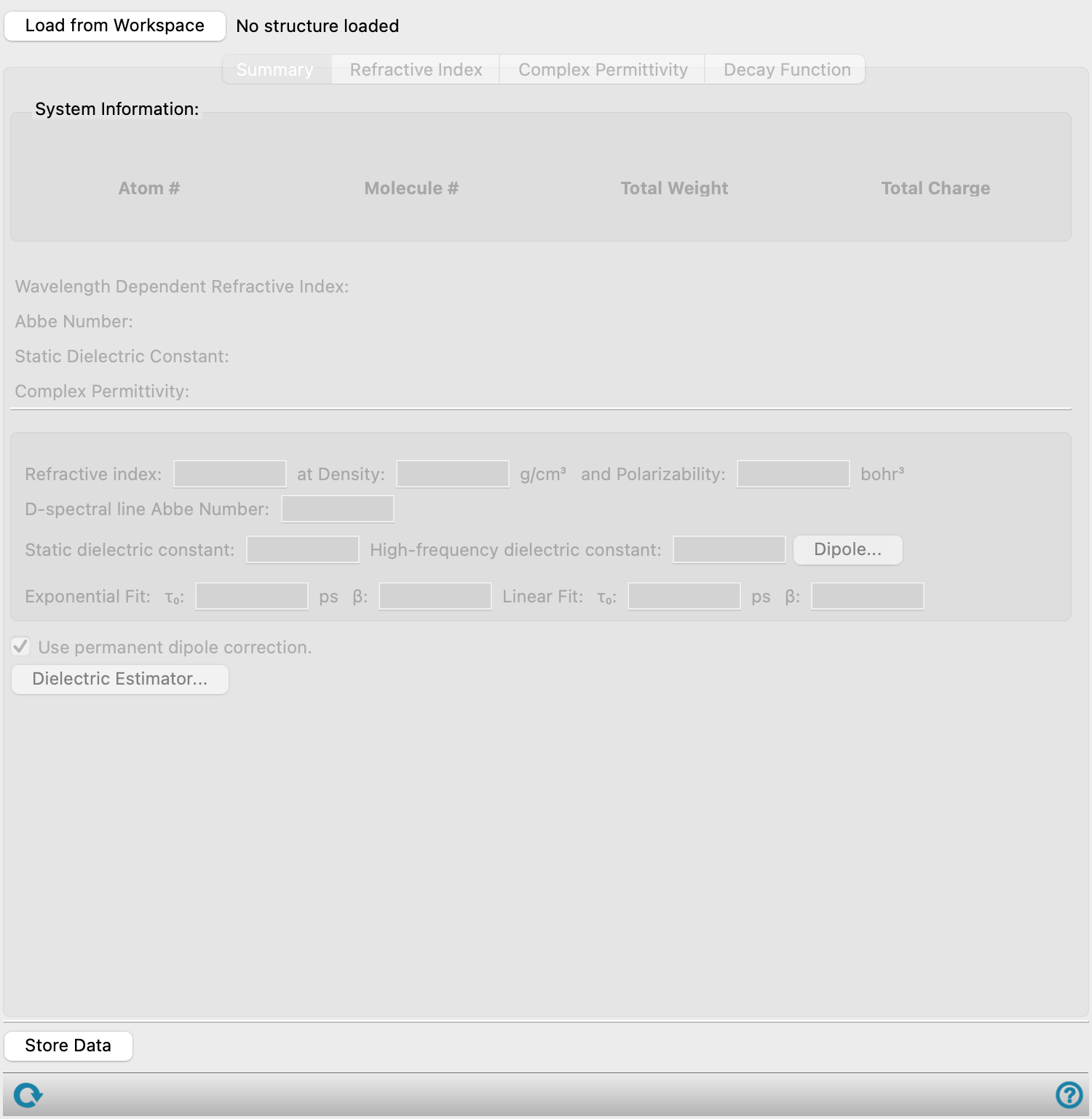
- Load from Workspace button
- Summary tab
- System Information section
- Wavelength Dependent Refractive Index text
- Abbe Number text
- Static Dielectric Constant text
- Complex Permittivity text
- Refractive index at Density and Polarizability text boxes
- D-spectral line Abbe Number text box
- Static dielectric constant text box
- High-frequency dielectric constant text box
- Dipole button
- Exponential Fit
- Linear Fit
- Use permanent dipole correction option
- Dielectric Estimator button
- Refractive Index tab
- Complex Permittivity tab
- Decay Function tab
- Store Data button
- Status bar
- Load from Workspace button
-
Load the data associated with the structure in the Workspace, which must be the output structure from a job run from the Amorphous Dielectric Properties Panel.
-
This tab displays the availability and value of various properties in noneditable text boxes, obtained from the simulation results and from the fitting of the dipole autocorrelation function from the MD simulations.
- System Information section
-
For the loaded structure, this section provides the number of atoms (Atom #), number of molecules or repeat units (Molecule #), Total Weight in atomic mass units, and Total Charge.
- Wavelength Dependent Refractive Index text
-
Displays Available if the Refractive index option was successfully calculated from the Amorphous Dielectric Properties Panel. When Unavailable, the Refractive Index tab is empty. Noneditable.
- Abbe Number text
-
Displays Available if the Abbe number option was successfully calculated from the Amorphous Dielectric Properties Panel. When Unavailable, the D-spectral line Abbe Number text box is empty. Noneditable.
- Static Dielectric Constant text
-
Displays Available if the Static dielectric constant option was successfully calculated from the Amorphous Dielectric Properties Panel. When Unavailable,the Systemwide Dipole dialog box opened by the Dipole button is empty. Noneditable.
- Complex Permittivity text
-
Displays Available if the Complex permittivity option was successfully calculated from the Amorphous Dielectric Properties Panel. When Unavailable, the Complex Permittivity tab is initially empty. Updating the fit in the Decay Function tab will recalculate the complex permittivity and update the plot in the Complex Permittivity tab. Noneditable.
- Refractive index at Density and Polarizability text boxes
-
Displays the refractive index calculated from the Lorentz-Lorenz equation, at zero frequency (i.e. using the static polarizability). The density and the polarizability values used in the equation are show in the text boxes. The volumetric density of the system is determined from the simulation in g cm-3. The isotropic static polarizability of a single molecule is calculated using Jaguar, in bohr3. Density and polarizability values can be set, for example to experimental values, using the Dielectric Estimator button. Corresponding properties, such as the refractive index, will be recalculated using the input density and polarizability values. Noneditable.
- D-spectral line Abbe Number text box
-
Displays the Abbe number (V-number, constringence) of the system. The refractive index at the Fraunhofer C, D1, and F wavelengths is used to calculate this value. Noneditable.
- Static dielectric constant text box
-
Displays the static dielectric constant, ε/ε0 at zero frequency. Noneditable.
- High-frequency dielectric constant text box
-
Displays the dielectric constant in the high-frequency limit. Noneditable.
- Dipole button
-
Opens the Systemwide Dipole dialog box, which lists the averaged dipole moments of each replicate in the x, y, and z directions as well as the standard deviation, in Debye.
- Exponential Fit
-
Displays the τ0 and β values for a exponential fit of the decay function.
Only editable when Exponential is selected for the Fitting Type option in the Decay Function tab. When this option is not selected, the values of τ0 and β displayed are calculated from the tau range chosen in the most recent exponential fit.
- τ0 text box
-
Displays τ0 from the Kohlrausch-Williams-Watts Function. τ0 is calculated from the exponential fit in the Decay Function tab. Changing the Upper Tau and Lower Tau values can change the fit and therefore the value of τ0. The value of τ0 is used to update the plot in the Complex Permittivity tab.
- β text box
-
Displays β from the Kohlrausch-Williams-Watts Function. β is calculated from the exponential fit in the Decay Function tab. Changing the Upper Tau and Lower Tau values can change the fit and therefore the value of β. The value of β is used to update the plot in the Complex Permittivity tab.
- Linear Fit
-
Displays the τ0 and β values for a linear fit of the decay function.
Only editable when Linear is selected for the Fitting Type option in the Decay Function tab. When this option is not selected, the values of τ0 and β displayed are calculated from the tau range chosen in the most recent linear fit.
- τ0 text box
-
Displays τ0 from the Kohlrausch-Williams-Watts Function. τ0 is calculated from the linear fit in the Decay Function tab. Changing the Upper Tau and Lower Tau values can change the fit and therefore the value of τ0. The value of τ0 is used to update the plot in the Complex Permittivity tab.
- β text box
-
Displays β from the Kohlrausch-Williams-Watts Function. β is calculated from the linear fit in the Decay Function tab. Changing the Upper Tau and Lower Tau values can change the fit and therefore the value of β. The value of β is used to update the plot in the Complex Permittivity tab.
- Use permanent dipole correction option
-
This option accounts for a non-zero dipole. This is helpful for systems with some remnant dipole, such as ordered systems. For systems with a dipole of zero, which typically occurs at long simulation times, this option should not be selected. The dipole correction is used by default.
- Dielectric Estimator button
-
Opens a dialog box in which values can be set in the Density text box, in g cm-3, and Polarizability text box, in bohr3. The panel enters Estimator Mode. Click on Estimate to update the properties in the Summary tab and plots in the other tabs update based on the inputs. Closing the dialog box exits Estimator Mode and returns the default data from the simulations.
-
Display plots of the refractive index or polarizability as a function of wavelength or frequency.
- Plot toolbar
-
The toolbar has tools for manipulating the plot and for saving images. The buttons that are common to all plot toolbars are described in the Plot Toolbar topic.
- Plot area
-
This area displays the plot of the x vs y axes chosen in the Type option menus.
- Type option menus
-
Choose the x and y axes to display in the plot. Options for the x axis are Wavelength or Frequency. Options for the y axis are Refractive Index or Polarizability.
-
Display plots of the complex permittivity in various forms, including the real and imaginary components, and loss curves.
- Results table
-
This table reports results from the complex permittivity plot for different fitting methods. Highlight a row to populate the plot area. The different columns are as follows:
-
Fitting Method—Displays the results from the complex permittivity plot for the corresponding fitting method. Choose between Exponential, Linear, and Custom fitting methods.
-
τ0—Displays τ0 from the Kohlrausch-Williams-Watts Function. τ0 is calculated from the corresponding fitting method in the Decay Function tab. Changing the Upper Tau and Lower Tau values can change the fit and therefore the value of τ0. The value of τ0 is used to update the plot in the Complex Permittivity tab. For fitting methods not currently selected, the value of τ0 displayed is calculated from the tau range chosen in the most recent use of that fitting method.
-
β—Displays β from the Kohlrausch-Williams-Watts Function. β is calculated from the corresponding fitting method in the Decay Function tab. Changing the Upper Tau and Lower Tau values can change the fit and therefore the value of β. The value of β is used to update the plot in the Complex Permittivity tab. For fitting methods not currently selected, the value of β displayed is calculated from the tau range chosen in the most recent use of that fitting method.
-
Dielectric Loss Peak Position—The frequency value for the maximum of the dielectric loss peak, in GHz.
-
Frequency—Enter a frequency, in GHz, to display the real and imaginary parts of the complex permittivity (Epsilon) values at that specified frequency.
-
Epsilon (Real)—The real component of the complex permittivity at the specified frequency.
-
Epsilon (Img)—The imaginary component of the complex permittivity at the specified frequency.
-
- Plot toolbar
-
The toolbar has tools for manipulating the plot and for saving images. The buttons that are common to all plot toolbars are described in the Plot Toolbar topic.
- Plot area
-
This area displays the plot chosen from the Type option menu.
- Type option menu
-
Choose the type of plot, from Magnitude vs Frequency, Complex Plane, and Loss Tangent.
- Export Data button
-
Export the frequency (in Hz), real component of the complex permittivity [Eps (Real)], and imaginary component of the complex permittivity [Eps (Imaginary)] to a CSV file. Opens a file selector so you can navigate to a location and name the file.
-
Plots the dielectric decay function against tau, with the option to adjust the range of tau values used for the complex permittivity function and the property values derived from it.
- Results table
-
This table reports results from the complex permittivity plot for different fitting methods. Highlight a row to populate the plot area. The different columns are as follows:
-
Fitting Method—Displays the results from the complex permittivity plot for the corresponding fitting method. Choose between Exponential, Linear, and Custom fitting methods.
-
τ0—Displays τ0 from the Kohlrausch-Williams-Watts Function. τ0 is calculated from the corresponding fitting method in the Decay Function tab. Changing the Upper Tau and Lower Tau values can change the fit and therefore the value of τ0. The value of τ0 is used to update the plot in the Complex Permittivity tab. For fitting methods not currently selected, the value of τ0 displayed is calculated from the tau range chosen in the most recent use of that fitting method.
-
β—Displays β from the Kohlrausch-Williams-Watts Function. β is calculated from the corresponding fitting method in the Decay Function tab. Changing the Upper Tau and Lower Tau values can change the fit and therefore the value of β. The value of β is used to update the plot in the Complex Permittivity tab. For fitting methods not currently selected, the value of β displayed is calculated from the tau range chosen in the most recent use of that fitting method.
-
- Fitting Type option
-
Choose between an Exponential or Linear fit for the decay function against tau.
- Plot toolbar
-
The toolbar has tools for manipulating the plot and for saving images. The buttons that are common to all plot toolbars are described in the Plot Toolbar topic.
- Plot area
-
This area displays the plot of the dielectric decay function against tau. You can adjust the range of tau values used for the Kohlrausch-Williams-Watts fitting of the dipole autocorrelation, by dragging the vertical dotted lines on the plot. The values in the limit text boxes are updated, the plot in the Complex Permittivity tab is updated as are the constants derived from it.
- Lower Tau and Upper Tau text boxes
-
Lower and upper limits of tau (in ns) for the fitting of the Kohlrausch-Williams-Watts function, which is used to obtain the complex permittivity. Changing the values changes the position of the vertical lines on the plot and vice versa.
- Store Data button
-
Save the property values at the current density and fitting range as a Project Table property.
- Status bar
-
The status bar displays information about the current job settings and status for the panel. The settings includes the job name, task name and task settings (if any), number of subjobs (if any) and the host name and job incorporation setting. The job status can include messages about job start, job completion and incorporation.
Use the Reset button
 to reset the panel to its default settings and clear any data from the panel.
 The status bar also contains the Help button
 , which opens the help topic for the panel in your browser. If the panel is used by one or more tutorials, hovering over the Help button displays a
  button, which you can click to display a list of tutorials (or you can right-click the Help button instead). Choosing a tutorial opens the tutorial topic.