Amorphous Dielectric Properties Panel

Using the Amorphous Dielectric Properties Panel

The calculation of dielectric properties can be run for multiple single molecules or multiple replica of pre-built disordered systems (CMS). For each single molecule input, a simulation cell is constructed with the specified number of molecules, using the Disordered System Builder. Pre-built disordered systems skip the simulation cell construction and are used as is for property calculations. For pre-built systems, we do not calculate refractive index or Abbe number.

The least accurate part of the process is the fitting of the dipole autocorrelation function. The accuracy of this function can be improved by increasing the simulation time and running more replicates of the system. Replicates can be distributed across GPUs (in the Job Settings Dialog Box), one for each replicate. The resulting properties (density, volume, dielectric decay parameters, etc.) are averaged across replicates, to give mean values and standard deviations. However, the longer the simulation time, the more replicates you add, and the smaller the recording interval, the larger is the disk space needed. You might need to find a balance between each of these parameters to prevent exceeding disk space capacity.

You can view plots of the results and adjust the fitting range in the Amorphous Dielectric Properties Viewer Panel.

Results are stored as Maestro properties, added to the structure. For the calculation of the refractive index and Abbe number only, the properties (with units) are

• Electric Polarizability (bohr³) (both static and finite-frequency)
• Refractive Index
• Abbe number
• Density (g cm⁻³)
• stdev Density (g cm⁻³)
• Temperature(K)
• stdev Temperature(K)
• Relative Permittivity inf (permittivity at high frequency)
• Wavelength Refractive Index File

When static and complex permittivities are calculated, the additional properties are

• Relative Static Permittivity
• Dipole Susceptibility
• Kww Beta (ps)
• Kww Tau
• Dipole Time Serial File
• Dipole Autocorrelation File
• Angular Frequency of Maximum Dielectric Loss (Hz)

The file properties are the paths to files containing the data described by the property name.

To write out the input file and a script for running the job from the command line, click the arrow next to the Settings button and choose Write. For information on command usage and options, see permittivity_driver.py Command Help.

 

Relevant formulae for the calculation of dielectric properties are shown below:

The refractive index n is calculated from the Lorentz-Lorenz equation,

where M is the molecular weight and N_A is Avogadro's number. The static polarizability α (and dynamic polarizability α(ω), where needed) is calculated with Jaguar. This is done on a range of oligomers if a polymer is built for the calculations, and the polarizability of the polymer chains is found from a linear fit. The number density ρ is determined from MD simulations with the OPLS4 force field.

The Abbe number (optical dispersion) is calculated from the frequency-dependent refractive index at the usual Fraunhofer C, D1, and F spectral lines (656.3 nm, 589.3 nm, and 486.1 nm),

The static permittivity is calculated from

The high-frequency permittivity ε_∞ is calculated using the Clausius-Mossotti relation,

where N is the number density of the molecule or repeat unit. The relaxation amplitude Δε is taken to include only the orientation polarization, evaluated from MD simulations of the dipole autocorrelation function, and is given by

where M is the dipole moment of the unit cell, V is the volume of the unit cell, and k_B is the Boltzmann constant.

The complex permittivity is calculated from

where Φ(t) is the dielectric decay function, and can be calculated from the autocorrelation of the dipole moment M over the trajectory. The trajectory data for the dielectric decay function is fitted to the Kohlrausch-Williams-Watts (KWW) function,

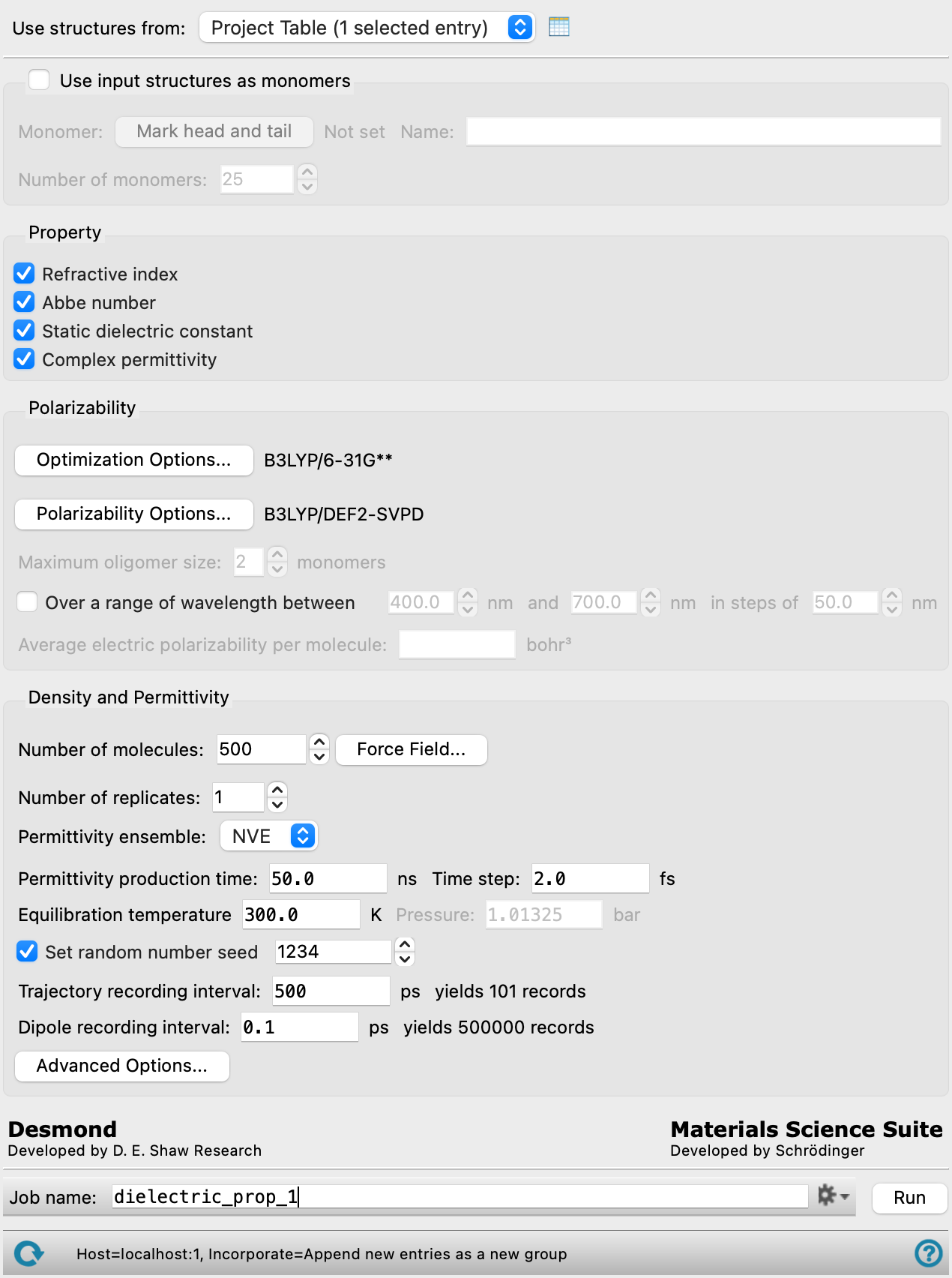
Amorphous Dielectric Properties Panel Features

Use structures from option menu

Choose the structure source for the dielectric property calculations. The structures must be single molecules.

• Project Table (n selected entries)—Use the entries that are currently selected in the Project Table or Entry List. The number of entries selected is shown on the menu item. An icon is displayed to the right which you can click to open the Project Table and select entries.
• Workspace (n included entries)—Use the entries that are currently included in the Workspace, treated as separate structures. The number of entries in the Workspace is shown on the menu item. An icon is displayed to the right which you can click to open the Project Table and include or exclude entries.

Open Project Table button

Open the Project Table panel, so you can select or include the entries for the structure source.

Use input structures as monomers option and section

Create a polymer of a defined length from monomers. The Polymer Builder Panel code is used to build the polymers.

Mark head and tail button

Mark the head and tail of the monomer for the polymerization. Opens the Mark Monomer Head and Tail Panel.

Name text box

Specify the name of the polymer.

Number of monomers text box

Specify the number of monomers used to create the polymer.

Property section

Choose the properties that are to be calculated, from the following. The tasks run by the job depend on the choices made.

• Refractive index
• Abbe number
• Static dielectric constant
• Complex permittivity

Polarizability section

Specify the protocols used for the quantum mechanical geometry optimization and the production calculations of the polarizabilities.

Optimization Options button

Set Jaguar options for the optimization of the geometry of the molecules, in the Optimization Options - Amorphous Dielectric Properties Dialog Box. Geometry optimizations are mandatory.

Polarizability Options button

Set Jaguar options for the calculation of the polarizability, in the Polarizability Options - Amorphous Dielectric Properties Dialog Box.

The basis set you choose in this dialog box is used for the calculation of the static polarizability, which is used for both the refractive index and the permittivity. It is critical to include polarization functions (**) and helpful to also include diffuse functions (++) in the basis set for the polarizability; it is also important that the basis set is not too small. The default basis set produces high quality polarizabilities when compared with experiment.

Maximum oligomer size text box

Specify the maximum size of oligomer for which QM calculations will be run, when creating a polymer from monomers. These oligomers are used to fit the polarizability as a function of the number of repeat units. The oligomer polarizabilities are reported in the log file.

Not available if Use input structures as monomers is not selected.

Over a range of wavelengths between N nm and M nm in steps of K nm option and text boxes

Specify a set of evenly spaced wavelengths for calculation of frequency-dependent polarizabilities. This allows you to calculate the optical dispersion (V-number) at wavelengths other than the standard set used for the Abbe number.

Average electric polarizability text box

Specify the average electric polarizability for the system. This is used to compute the high frequency dielectric constant. Only available for pre-built Desmond model systems (CMS).

The maximum specified electric polarizability must be less than where ρ is the number density determined from MD simulations.

Density and Permittivity section

Make settings for the production MD simulations for the density and the dipole autocorrelation function, from which the permittivities are calculated.

Number of molecules text box

Number of polymers text box

Specify the number of molecules or polymers to use when building the system for simulation. The option text and the default value depends on the choice for Use input structures as monomers.

Force Field button

Click the Force Field button to specify the force field to use and any custom charges, in the Force Field Dialog Box. The current force field is shown to the left of the button. Learn more about available force fields in the OPLS Force Fields and Machine Learning Force Fields documentation. Setting custom charges may improve the calculated dipole moments and hence the dielectric properties.

Number of replicates text box

Specify the number of replicates of the system to use for averaging, when complex permittivity is requested. The density, static permittivity, and complex permittivity from dipole auto-correlation are obtained by averaging over the replicates. More replicates provides better statistics for the averaging, at the cost of more MD simulations and larger disk space usage. The replicates can be distributed across GPUs.

Density ensemble option menu

This menu is shown if Static dielectric constant and Complex permittivity are not selected. Only the NPT ensemble is available, and it is grayed out, as the NPT ensemble is required. The simulations are performed solely to obtain the density. The ensemble selected here is for the production simulations; the equilibration protocol is done in multiple stages with different ensembles and conditions.

Permittivity ensemble option menu

Choose the ensemble class from this option menu. The following classes are available:

• NVE—constant particle number (N), volume (V) and energy (E). This class represents the microcanonical ensemble.
• NVT—constant particle number (N), volume (V) and temperature (T). This class represents the canonical ensemble.
• NPT—constant particle number (N), pressure (P) and temperature (T). This class is an isothermal-isobaric ensemble, the common experimental conditions.

This menu is shown when Static dielectric constant or Complex permittivity is selected (or both), and includes the NVE and NVT ensembles. The ensemble selected here is for the production simulations; the equilibration protocol is done in multiple stages with different ensembles and conditions.

Density production time text box

Permittivity production time text box

Specify the desired simulation time in ns. This is the time for the simulation from which the permittivity properties are evaluated. Long simulation times provide better accuracy for the dipole autocorrelation function. The default is 50 ns.

Time step text box

Specify the time step for the simulation in fs.

Trajectory recording interval text box

Set the recording interval for saving points on the trajectory, in ps. The resultant number of records to be written is reported to the right.

Equilibrium temperature text box

Specify the equilibrium temperature of the system, in kelvin. This temperature is the target for the equilibration process that is performed prior to the production simulations. It is not relevant for simulations in the NVE ensemble, but it does specify the temperature in the NVT ensemble.

Pressure text box

Specify the pressure to be used, in bar. Not available for the NVE and NVT ensemble classes.

Set random number seed option and text box

Select this option to specify a random seed to be used in the simulations. Specifying the seed allows you to reproduce the results, unless other factors affect them. If this option is not selected, a seed is chosen at random.

Dipole recording interval text box

Set the recording interval in ps for saving the system dipole moment, for the purpose of calculating the dipole autocorrelation function. This is the amount of time between frames in the trajectory. The entered value is rounded to an integer multiple of the far time step size. The resultant number of records to be written is reported to the right. Only available if Static dielectric constant or Complex permittivity is selected.

Advanced Options button

Opens the Amorphous Dielectric Properties — Advanced Options Dialog Box.

Job toolbar

Manage job submission and settings. See Job Toolbar for a description of this toolbar.

The Job Settings button opens the Amorphous Dielectric Properties - Job Settings Dialog Box, where you can make settings for running the job.

Status bar

Use the Reset button to reset the panel to its default settings and clear any data from the panel. If the panel has a Job toolbar, you can also reset the panel from the Settings button menu.

If you can submit a job from the panel, the status bar displays information about the current job settings and status for the panel. The settings include the job name, task name and task settings (if any), number of subjobs (if any) and the host name and job incorporation setting. The job status can include messages about job start, job completion and incorporation.

The status bar also contains the Help button , which opens an option menu with choices to open the help topic for the panel (Documentation), launch Maestro Assistant, or if available, choose from an option menu of Tutorials. If the panel is used by one or more tutorials, hover over the Tutorials option to display a list of tutorials. Choosing a tutorial opens the tutorial topic.

Related Topics

• Amorphous Dielectric Properties Viewer Panel
• Polymer Builder Panel
• Mark Monomer Head and Tail Panel
• Disordered System Builder Panel
• Amorphous Properties Panel
• permittivity_driver.py Command Help.
• Amorphous Dielectric Properties — Advanced Options Dialog Box
• Amorphous Dielectric Properties - Job Settings Dialog Box