Selecting Martini Parameters

The Martini force field[1] is one of the most widely used coarse-grained force fields. This is in part due to the availability of parameters, validation, use, and extension by many groups, along with a rational and comparatively simple parameterization approach. What is described here is based largely on a reference from Bereau and Kremer [2].

The Materials Science coarse-grained modeling infrastructure for the Martini force field supports small molecules, some types of polymers, and proteins. RNA, DNA, and carbon nanostructures are not supported by the current infrastructure. Please note that the Martini force field is only supported on GPUs and will not run on CPUs.

This topic describes how to map an all-atom molecule onto a Martini coarse-grained one, the standard site types for the Martini force field, how to select the types to use for your molecule, and how to choose force-field parameter values.

Choosing a Mapping

Choosing a mapping from all atoms into coarse grained sites involves dividing up the molecule into groups of about 4 heavy atoms (and hydrogen atoms bound to them) for linear segments and about 2 heavy atoms for rings. There are often multiple ways to do this well, so there is flexibility in the choice. Usually, one wants the surface of the coarse-grained molecule to roughly follow the surface of the corresponding atomistic model, have coarse-grained sites which map onto small reasonably compact groups of atoms, and the coarse-grained sites should be able to collectively represent any important flexibility or rigidity that the molecule has.

The MSG installation has a number of coarse-grained sites already defined (listed in the Site Types for Martini topic). If a simulation includes a molecule containing coarse-grained sites not covered within the installation, new coarse-grained site types can be developed. During this process it helps to keep in mind the standard Martini site types and perhaps the types of molecules or molecular fragments that are already available in the installation (see below). Using existing general types will minimize the effort required to simulate a new system.

Standard Martini Site Types and Nonbonded Interactions

All particle types have the same Lennard-Jones 12-6 + Coulomb potentials, and the standard shift function of GROMACS is used [3]. Table 1 briefly describes the standard Martini types. Table 2 gives the Lennard-Jones parameters for the different types of sites.

Roman numerals from 0 to IX denote different combinations of Lennard-Jones σ_ij and ϵ_ij parameter values. All σ_ij are 4.7 Å except for type IX where it is 6.2 Å. The ϵ_ij values are given in Table 3 below.

Standard Modifications to Martini Types

Many of the standard interactions types can be modified for particular needs. The modifications include:

Antifreeze water BP₄ particles

To avoid problems with freezing of pure Martini water (P₄), aqueous Martini simulations typically include modified water particles ("antifreeze water") for about 10% of the water particles. These BP₄ particles are just like P₄ particles except that σ and ϵ for the P₄(water only)-BP₄ interaction are increased to 5.7 Å (instead of 4.7 Å) and 5.6 kJ mol⁻¹ (1.334 kcal mol⁻¹, instead of 5.0 kJ mol⁻¹).

Rings

To mimic the shape and stiffness of rings a finer resolution is used; typically 2 heavy atoms per Martini site. For instance, 6-membered all-atom rings such as cyclohexane or benzene are often represented by 3 coarse-grained sites in a ring. The site types are based upon the normal site types except that smaller σ values (4.3 Å) and smaller well depths (75%) for small-particle - small-particle interactions are used. The new types have an 'S' before the site type that they are based on. Note that ring-nonring interactions are handled without the reductions in σ and ϵ, e.g., benzene is presented by a triangle of SC₅ sites. Benzene-benzene interactions use the 'S' adjustments while benzene - butane interactions use the normal parameters for C₅ - C₁ sites.

Special cases

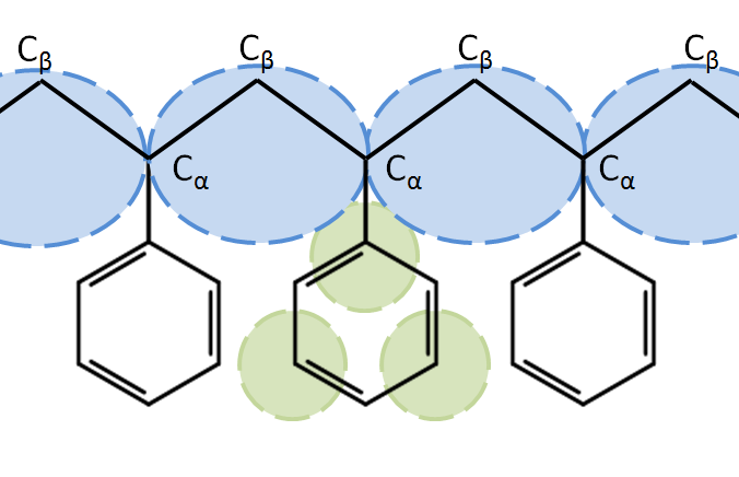
For specific compounds the Martini force field has been extended to attain better accuracy. One collaboration by Rossi and Montecelli has produced many such models, e.g., a model for polystyrene[4], using 3 SC_4ps for the phenyl group. In cases like this the new bead type is often based upon a standard type with only a few modifications to a small subset of the interactions.

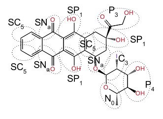
Complication: Site Types in Molecules

Martini site types are fairly general and may be used in different topologies even within the same molecule. As a result the same type of Martini site may have different valence parameters in different usages. This leads to the use of two levels of site types:

• Martini site types
• Site types in molecules

For instance for cholesterol, depicted here atomistically and with a Martini representation,

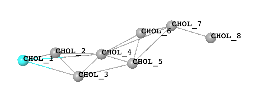
several different sites map onto the same Martini site type, as shown in the table below.

Selecting Martini Site Types for Your Molecules

Ways to select site types:

1. Look in the collection of site types/molecule fragments available (listed in "Site Types for Martini Help" topic in Maestro) for drawing molecules in the Coarse Grained sketcher to select site types in molecules. Alternatively, if you are using standard types of molecules, whole coarse-grained molecules can be imported using the "Import Coarse Grain Structures" panel in Maestro.

2. If there is a fairly direct correspondence with standard Martini types, e.g., a saturated hydrocarbon chain can be broken up into -(CH₂)₄- segments you can just select that Martini site type in the force field panel.

3. Calculate logP for oil/water partitioning using various tools including MSS (ALOGPS is the one that the Martini group uses, http://146.107.217.178/web/alogps/ - accepts SMILES strings) for small molecules containing the groups of atoms and select the Martini site type with a similar known logP value (see Table 3 below). Examples for such selections are given in Table 5.

4. More accurate treatments (potential future development).

You can elect to create a new custom Martini site type however you will need to choose the non-bonded parameters with care.

Note that the Martini parameters for P₁ are similar to those for N_da.

AlogP can be generated in the Maestro Project Table, as follows:

1. Select the desired entries.

2. Choose Data → Add Properties → Standard Molecular Property.

3. Select AlogP. An AlogP column is added to the Project Table containing the calculated values.

4. Multiply the AlogP value by −1.37 to estimate the O/W partitioning free energy at 300K.

Creating Martini Molecules

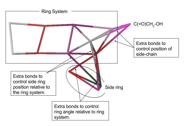
If the molecule already exists in the database for Martini (see "Import Coarse Grain Structures" panel in Maestro) we recommend that you use that structure as it will have predefined site types and valence parameters. Otherwise where possible draw in the new coarse-grained molecules using the Coarse-Grained Sketcher. For groups directly attached to fused ring-systems draw in extra bonds (in the Coarse Grained sketcher) to control the position of those groups relative to the ring rather than eventually using angle potentials. For instance, for annamycin the addition of extra bonds to control the relative position and orientation of the groups relative to the main ring system is helpful and also a more robust approach than using bond angles or torsions for this purpose.

Choosing Parameters

The project goals and timelines will strongly influence the strategy that should be used to select Martini parameters.

Non-bonded parameters

The major strength of the Martini force field is that what is normally the hardest part of parametrizing a coarse-grained force field for a new type of site, determining the non-bonded interactions, can often be replaced by an easier problem, selecting an appropriate the Martini site type. Currently, we do not have tools to help with determining non-bond potentials. Luckily, in addition to the standard Martini site types there are quite a few specialized ones in the literature, e.g., for PEO, Polystyrene, PAMAM, and a good source for information on these is available on the Martini website (http://cgmartini.nl/index.php/force-field-parameters). When adding or using a non-standard Martini site type in a more complex system, please be careful to check that all of the non-bonded interactions have appropriate parameters. For instance, there are special SP0 and SPh Martini site types for PEG/PEO; however, not all of the nonbonded interactions of these sites have been specified in the standard force field file and they will be assigned default values in the GUI. These unspecified values are listed as Guess values in the Nonbonded tab of the Assign Force Field panel. Please note that only sites with Martini sites-types of Qda, Qa, Qd, and Q0 can carry non-zero charges.

Valence parameters

The following functional forms are supported for valence potentials for the Martini force field:

Exclusions:

Martini potentials exclude non-bonded interactions between sites that are bonded to each other or within the same ring system.

Risks associated with angle potentials:

Angle potentials with θ_eq not equal to 0 or 180° and with a k value small enough that 0 or 180° angles will be sampled may cause Desmond to halt with an error because the force is finite but its direction is undefined. Dihedral angles φ are defined using 4 atoms i, j, k, l to identify two planes defined by i, j, k and j, k ,l. If i, j, k or j, k, l become collinear the corresponding plane cannot be defined and the torsion angle is undefined; something that may cause Desmond to halt with an error.

Choosing valence parameters

If you built your molecules using sites from the provided set of the site types in molecules provided in the installation, in addition to getting non-bonded parameters you also get many or all of the valence parameters. You can mix and match to some extent from this dataset. For example, C₁₂E₆ can be thought of a hydrocarbon chain represented by BUT sites for the hydrocarbon attached to a PEG-like chain composed of SPO plus a terminal SPh. The valence parameters in the chain will be provided from the database. The user is responsible for specifying any of the missing bond, angle and torsional parameters involving sites from both chains where they are connected. It can be useful to do a MacroModel conformational search on the all-atom molecule or portions thereof to get information on local geometry. The following recipe for valence interactions may be helpful:

• For normal sized sites (4 heavy atoms) in linear parts of the molecule use:

  • a default bond length of 4.7 Å with a force constant of 2.988 kcal mol⁻¹ Å⁻² (the Assign force field panel will use these values by default). If you prefer you can use a distance based upon the all-atom geometry provided by MacroModel or from a molecular dynamics simulation.

  • Bond angle potentials, torsional potentials, improper torsions are not created by default. In most Martini force fields these are used as needed. Bond angle potentials are used moderately frequently to maintain stiffness (e.g., persistence length). Default values for angle potentials use a bond angle based upon molecular geometry (e.g., in an alkane it is 180° in more complex species the geometry from MacroModel or other types of calculations may be used at your discretion) with a force constant of 5.975 kcal mol⁻¹. Torsions and Improper potentials are most commonly used to control the geometry of rings, particularly, fused rings.

• For valence interactions between small and normal sized sites follow the rules given above.

• For valence interactions between small sites follow the rules above except:

  • Use a shorter bond length by default: 4.3 Å and a larger force constant (11.950 kcal mol⁻¹ Å⁻²)