MxMD Analysis
The primary means of analyzing an MxMD simulation is by inspecting the hotspots of each cosolvent probe.
Visualizing MxMD Results
The output of a MxMD simulation is a compressed Maestro project archive mxmd_job.prjzip. In addition to the project archive, a mxmd_job_results/ directory is created. The directory contains:
- Maestro files (
.mae) with the last frame from each simulation for each cosolvent probe and corresponding volumetric data with density information for each probe type (in Xplor-formatted.cnsfiles). - The probes corresponding to each hotspot in Maestro files
hotspot_X.mae. .cms/.xtc trajectory frames for each probe type. The contents of the systems will be solute (receptor) only.
These files allow a further insight into the distribution and orientation of the cosolvent probes.
You can run the trajectory_binding_site_id.py script to identify transient binding sites.
You can load the output into Maestro directly by choosing File → Open Project or pressing Ctrl+O (⌘O). The Open Project project selector opens, in which you can navigate to and select the project file.
You can also view results with the View result option in the Mixed Solvent MD Panel. A table with all the probe hotspots is listed, and you can view hotspots in the Workspace. The probe hotspots are displayed as surfaces with a cutoff of 20 σ.
Analyzing Cosolvent Occupancies
For each probe, frames from the production stages are extracted for all trajectories (10 by default) and aligned with the input coordinates. The occupancy of the functional groups of the cosolvent probes are calculated on a 0.5 Å grid. For probe molecules with multiple functional groups, the occupancies of all functional groups are evaluated individually. The raw bin counts,Xxyz for each grid point are converted to Z-scores:

where <X> is the mean of all the raw bin counts and σ is the standard deviation [4]. The output maps are contoured at an isovalue of 20σ. This value can be changed when visualizing the results.
Detecting and Scoring Hotspots
Hotspots can be used to identify and prioritize density regions of biological interest within the protein or DNA/RNA structures. Each probe’s occupancy map is clustered via single-linkage hierarchical clustering with a cutoff of 3.0 Å. Each cluster forms a spot. Overlapping clusters are merged into hotspots. A hotspot consists of at least two overlapping spots. The MxMD score for a hotspot is calculated by summing the Z-scores over all grids, overlapping spots, and probes.

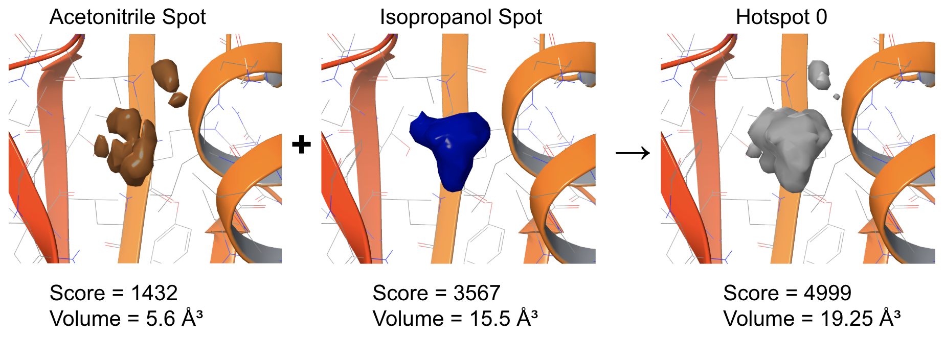
Figure 1: Illustration of the hotspot detection. First, occupancy maps of probes are clustered into spots. Then, overlapping spots across all probes are merged into hotspots.