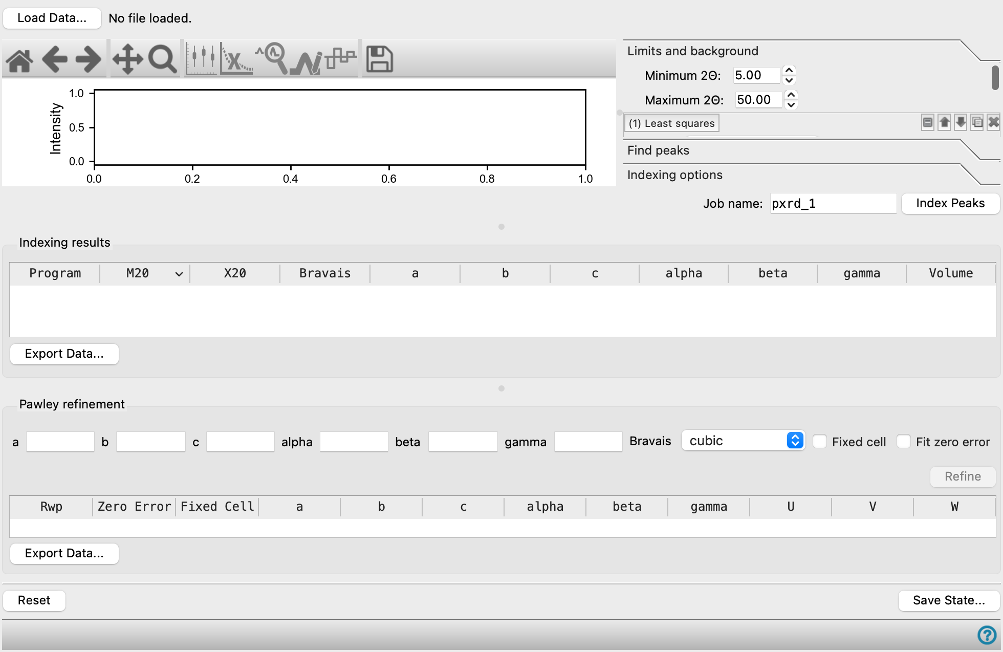
Powder Diffraction Indexing Panel
Locate peaks in a plot of intensity against angle from an x-ray powder diffraction experiment, after removing background, assign Miller indices to them, and use this data to determine the lattice parameters. Peaks can be detected automatically and adjusted or assigned manually. The lattice parameters can be refined based on the indexing results.
To open this panel: click the Tasks button and browse to Materials → Tools → Powder Diffraction Indexing.
The following licenses are required to use this panel: MS Maestro
- Using
- Features
- Additional Resources
Using the Powder Diffraction Indexing Panel
The first task after loading some experimental data is to perform a background subtraction, which you do in the Limits and background tab. There are tools for defining the background automatically and by manual adjustment of a spline fit. It is a good idea to perform an automatic fit first, which gives a base curve that you can adjust manually. The automatic fit can be done with three different algorithms, and you can use any of the three in multiple steps to successively remove residual background. Once you have the base curve, click the Edit Splines button or the Fit splines toolbar button and drag the spline points to adjust the background. Subtracting the background is important for the peak search, as it can eliminate the identification as peaks of many fluctuations in the background whose amplitude is small.
The next task is to identify the peaks. As for the background subtraction, there is an automatic algorithm that finds peaks, and you can add and adjust peaks manually. The peak detection algorithm has some tolerances for where the noise level is and whether peaks are too close to be considered as separate peaks. Peaks that are closer than the tolerance are merged into a single peak placed at the intensity-weighted average location. You may need to adjust these tolerances to get the optimum selection of the real peaks while eliminating those that are noise. If there are too few peaks identified, you may have to decrease the tolerance value; if too many, increase it. Click the Find Peaks button or the Search for peaks toolbar button to perform the search. Peaks are marked with vertical blue lines, and reported in the table in the Find peaks tab. It is likely that you will need to do manual selection and adjustment after the automatic search. Click the Edit peaks toolbar button to manually select and drag existing peaks or click to add new peaks. For precise manual selection of a peak position on the plot, you might want to zoom in on a region of the plot, which you can do with the toolbar buttons, then zoom out again. You can also edit the peak positions in the table, and they are updated in the plot.
The next task is to perform the indexing and check the results. There are options to choose the Bravais lattices, limit the cell parameters and the fit of the calculated peaks to the identified peaks. The indexing is performed with the available programs. NTreor is included in the software installation. DICVOL06 and DICVOL91 can be used but must be downloaded and installed. See Installing DICVOL for Powder Diffraction Indexing for instructions.
The final task is to refine the cell parameters based on the indexing results, using the Pawley refinement method.
Powder Diffraction Indexing Panel Features
- Load Data button
- Limits and background tab
- Find peaks tab
- Indexing options tab
- Job name text box
- Index Peaks button
- Indexing results section
- Pawley refinement section
- Save State button
- Plot toolbar
- Plot area
- Reset button
- Load Data button
-
Load powder diffraction data, and also load settings, peaks, background and results from use of the panel. Opens a file selector to locate and load the file. The allowed file types are:
- Panalytical (
.xrdml) - Bruker raw (
.raw), version 3 - FullProf (
.dat) - Topas (
.xye) - Diffraction pattern indexing (
.pxrd) - Raw data (
.xy), just 2Θ and intensity.
The last of these contains the data from a saved state, which includes the raw data and the data generated from the panel, such as background curve, peak positions and intensities, etc.
- Panalytical (
- Plot toolbar
-
The toolbar has tools for manipulating the plot and for saving images. The buttons that are common to all plot toolbars are described in the Plot Toolbar topic.
-
In addition, the toolbar has several buttons that are specific to the peak specification task.

Fit splines: Fit the background curve using a set of splines, and adjust the spline points by dragging. The number of points is specified in the Number of spline points text box.
This button does the same as the Edit Splines button.
Subtract background: Click to view the plot after background subtraction; click again to view the plot with the background present (and marked as a red line). When searching for peaks, many small fluctuations in the background can be identified as peaks when the background is not subtracted: these additional peaks are usually spurious. 
Search for peaks: Run a search for peaks in the current plot, using the settings in the Find peaks tab. The peaks are marked with vertical blue lines.
This button does the same as the Find Peaks button.
Edit peaks: Edit the peaks in the plot manually.
- Click on a peak to add a peak.
- Click and drag to reposition a peak.
- Double-click to remove a peak.

Difference plot: Display a difference plot between the experimental and predicted curves. Both the full curve and the difference curve are displayed, along with the peak position markers. - Plot area
-
The plot shows the x-ray intensity as a function of 2Θ. You can click on the plot to mark the position of a peak (with a vertical line), and drag the peak markers to reposition them.
- Limits and background tab
-
Specify limits on 2Θ and specify methods for background subtraction.
- Minimum 2Θ text box
-
Specify the minimum value of 2Θ to use for background fitting and peak detection. The data in the plot is updated to reflect this range when you calculate the background.
- Maximum 2Θ text box
-
Specify the maximum value of 2Θ to use for background fitting and peak detection. The data in the plot is updated to reflect this range when you calculate the background.
- Filtering tools
-
These tools apply a filter that subtracts the background and returns the data with the background subtracted. It is usually only necessary to use one filter, but sometimes this is not enough to remove the background. You can specify several filtering steps, which are applied sequentially: the output from one filter step is passed to the next filter step to remove the residual background.
- filter step management buttons
-
These buttons perform display and ordering operations on the filter step. They allow for easy duplication and rearrangement of filter steps.


Show or hide the contents of the filter step. When hidden, only the filter step number, label (if any) and these buttons are displayed. This is useful when you have a number of filter steps and want to compare two separate filter steps, for example. 

Move the filter step up or down one place in the list. 
Duplicate the filter step. This is useful for creating similar filter steps with variations on the settings. 
Delete the filter step. - Method option menu
-
Choose the filter method, from
- Least squares—the most generally useful method.
- Rubber band—useful when there is a rising background at low 2Θ values; uses a convex hull.
- Savitzky-Golay—uses polynomial fitting of the data; for background subtraction, a larger window size and a small polynomial order gives better results. This method is usually used for peak fitting.
The other tools depend on the method chosen.
- Smoothness text box
-
Controls the window over which the smoothing is done and hence the smoothness of the background curve. Decrease this value if the background has more structure. Only available for the Least squares method.
- Y-shift factor text box
-
Scaling value for intensity values to produce a smooth curve. Increasing this value introduces more of the intensity into the smoothing. Only available for the Least squares method.
- Window size text box
-
Number of consecutive points used for fitting. Must be an odd integer. Only available for the Savitzky-Golay method.
- Polynomial order text box
-
Order of the polynomial used for fitting the data. Must be less than the window size. Only available for the Savitzky-Golay method.
- Add Filter Method button
-
Add a set of filter method tools below the last set.
- Calculate Background button
-
Calculate the background using the chosen methods. The background is marked on the plot.
- Edit Splines button
-
Fit the background curve using splines, and adjust the spline points by dragging them in any direction. This button does the same as the Fit splines toolbar button.
- Number of spline points text box
-
Specify the number of spline points used to fit the background curve.
- Find peaks tab
-
Find peaks in the plot. If you change any of the parameters, the peak detection is run automatically.
- Minimum peak separation text box
-
Specify the minimum distance between peaks in terms of the value of 2Θ. Two peaks will not be reported if they are separated by less than this amount; instead, the intensity-weighted average of the two peaks is reported as a single peak. This value is applied during the automatic detection of peaks.
- Minimum peak intensity text box
-
Specify the minimum absolute intensity for detection of a peak. The value is marked on the plot as a horizontal gray dashed line.
- Noise percentage text box
-
Specify the percentage of the intensity below which any data is considered noise. This percentage is applied to small regions that are defined dynamically during peak detection.
- Peak 2Θ tolerance text box
-
Tolerance for defining a peak. This value is used in two ways: first, it is used as a post-selection filter in the automatic peak detection. If the tolerance value is larger than the Minimum peak separation value, the peak with the lowest 2Θ value is chosen if peaks are closer together than the tolerance. Second, it is used for picking peaks in the plot. If you click within the tolerance value of an existing peak, the peak is selected; if you click further than the tolerance from an existing peak, a new peak is placed. If there are multiple peaks within this distance of where you click, the one with the smallest value of 2Θ is selected.
- Find Peaks button
-
Find peaks in the diffraction data using the parameters set above. The peaks are listed in the table below and marked on the plot. This is mainly useful at the beginning, and when you switch between showing the background and removing the background (with the Subtract background toolbar button).
- Peak table
-
This table lists the peaks that were found. You can select multiple rows to delete unwanted peaks. Selected peaks are marked with thicker blue lines in the plot. The peak position values can be edited to move the peaks. The intensity is the value of the intensity at the peak position, and changes as the peak is moved.
- Delete Selected Rows button
-
Delete the rows (peaks) that are selected in the peak table.
- Export Data button
-
Export the peak data to a CSV file. Opens a file selector for choosing a location and a file name.
- Indexing options tab
-
Set options for indexing the peaks and determining the lattice parameters. Peaks are predicted from the lattice and compared with the peaks identified in the search above.
- Indexing algorithm options
-
Select the options for the indexing algorithms you want to use. The indexing is performed with each of the selected algorithms. Options for DICVOL are available if you have the software installed.
- Bravais lattices for indexing options
-
Choose one or more lattice types for indexing, from Cubic, Tetragonal, Hexagonal, Orthorhombic, Monoclinic, and Triclinic.
- Cell parameter search options
-
Specify options for the search for possible values of the cell parameters.
- Max a, Max b, Max c text boxes
-
Specify the maximum allowed values of the a, b, and c lattice parameters, in angstroms.
- Min angle and Max angle text boxes
-
Specify the minimum and maximum values for any of the angle parameters (α, β, γ).
- Min volume and Max volume text boxes
-
Specify the minimum and maximum volume of the unit cell.
- Absolute error text box
-
Maximum error in 2Θ for the assignment of the peaks predicted from the lattice to the peaks identified in the search (input peak). If a predicted peak is within this amount of an input peak, the assignment is accepted.
- Minimum figure of merit text box
-
Minimum acceptable value of the figure of merit (M20) derived from the match between input and predicted peaks. Values of M20 below about 6 are generally considered to indicate a poor match to the identified peaks.
- Number of impurity peaks text box
-
Maximum number of identified peaks that are permitted to be missing in the predicted peak set, when the figure of merit is calculated. These peaks are ascribed to impurities. The number of impurity peaks is reported in the results table as X20.
- Zero point error options and text box
-
Choose a method for shifting the 2Θ coordinate to match predicted peaks (i.e. a shift in the location of the zero value of the 2Θ coordinate), and optionally specify a shift value. These options are only available when using the DICVOL06 and DICVOL91 programs. The Custom option is available for both DICVOL91 and DICVOL06, and you can specify a value. For DICVOL06 the Automatic option is also available, which automatically determines the zero point error. The NTreor program automatically determines the zero point error.
- Job name text box
-
Specify a job name for the indexing job. This allows you to identify the files that are associated with the particular diffraction data set.
- Index Peaks button
-
Run the peak indexing. A progress dialog box is displayed while the indexing is running, showing the location where the files are written, and reporting on progress. When the indexing is done, the Results table is populated with the parameters of the cells, ordered by the M20 figure of merit.
- Indexing results section
-
This section displays the results of the indexing and allows you to export the data.
- Results table
-
The table reports the unit cell parameters and information, and measures of the fit from the peak indexing. When you select a row, the predicted peaks are displayed in the plot, in dashed red lines, and the cell constants are entered into the text boxes in the Pawley refinement section.
Program
Program that generated the prediction. M20 Figure of merit, based primarily on the first 20 peaks (counting from 2Θ=0). Results with values below about 6 should be treated with caution. X20 Number of impurity peaks (i.e. lines that could not be indexed) Bravais Bravais lattice type for the unit cell a, b, c Unit cell axes alpha, beta, gamma Unit cell angles Volume Unit cell volume Laue Group Laue group for the cell. Changing this group changes the predicted peaks, and also the space group value. Trying different groups can help to choose the best unit cell for the experimental data. Space Group Space group corresponding to the Laue group. - Export Data button
-
Export data from the table to a CSV file. Opens a file selector for choosing a location and a file name.
- Pawley refinement section
-
Perform a Pawley refinement of the cell parameters. The refinement is performed on the indexing result selected in the Results table, above.
- Cell constant text boxes
-
These text boxes specify the input cell constants (a, b, c, alpha, beta, gamma) for the refinement, and are populated automatically when you select a row in the indexing results table. You can adjust the values; however if you make large adjustments, the refinement might take a long time, or even fail.
- Bravais option menu
-
Choose the Bravais lattice type for the refinement. The type is automatically selected when you select a row in the indexing results table.
- Fixed cell option
-
Select this option to fix the cell during the refinement. The peak profile parameters (U, V, W) are varied to fit the data, and the R factor is reported. This is useful to check the indexing results to locate the set that has the best fit, and then perform a refinement of the cell on that result with this option deselected.
If not selected, a Pawley refinement is run, in which the cell parameters are varied.
- Fit zero error option
-
Include the location of the zero value of 2Θ in the refinement, to obtain a better fit. This doess the same as the Zero point error option for indexing.
- Refine button
-
Run the refinement with the specified cell parameters and options. When the refinement finishes, a new row is added to the results table below.
- Refinement results table
-
This table presents the results of the refinement. You can select a row to display the predictions of the refinement in the plot. The errors in the predicted intensities are displayed by changing the color of the top part of the peak to indicate the error. You can also display a difference plot between observed and predicted intensities.
Rwp
Weighted profile R factor for the refinement. Ideally, this should be 10 or less for a "good" refinement. Zero Error
Value of the error in the zero of 2Θ from the refinement. This value is nonzero only if Fit zero error is selected. Fixed Cell Shows the status of the Fixed Cell option as True or False. a, b, c Unit cell axes alpha, beta, gamma Unit cell angles U, V, W Peak profile parameters - Export Data button
-
Export data from the table to a CSV file. Opens a file selector for choosing a location and a file name.
- Reset button
-
Reset the panel to its default settings, clearing all data.
- Save State button
-
Save the current state of the panel and data, including raw diffraction data, background fitting parameters and peak positions. Opens a file selector for choosing a location and a file name. The file extension is
.pxrd. Saved states can be imported in to the workflow with the Load Data button.