MS MD Trajectory Analysis Panel
Analyze a trajectory from a Desmond MD simulation and present information on bulk properties derived from the trajectory, such as plots of the density and the cohesive energy.
To open this panel, click the Tasks button and browse to Materials → Classical Mechanics → Trajectory Analysis → MS MD Trajectory Analysis.
You can also open this panel with the Workflow Action Menu  for results from a MD Multistage Workflow that contains at least one Minimization or Molecular Dynamics or Analysis stage.
- Using
- Features
- Additional Resources
Using the MS MD Trajectory Analysis Panel
The purpose of this panel is to display information about bulk properties derived from a simulation, in graphical form. The properties that can be displayed are volume, density, heat of vaporization, cohesive energy, and solubility parameter (including a breakdown into van der Waals and electrostatic contributions). The properties that are actually available for display depend on the choice of analysis properties you made in the simulation.
Note: For charged systems or systems calculation using machine learning force fields, the heat of vaporization, cohesive energy, and solubility parameter are not available.
To generate analysis data, you can click the Load button and select an output -out.cms file that has an associated trajectory, and run the analysis. Once the analysis is run, you can load the event analysis file (.eaf or .st2) either with the Load button, or by including the structure in the Workspace and clicking Load from Workspace. You can then examine the various graphical representations of the bulk properties.
If you run the simulations with the MD Multistage Workflow Panel, you can add analysis stages to the workflow that generate .eaf files. For example, you could run simulations at a range of temperatures and do an analysis at each temperature. The Crystal Morphology Calculations Panel also produces .eaf files.
You can create a PDF file that contains all the charts in the panel, along with explanatory text and tables, or you can export just the charts as images. You can also export the data to a plain text file if you want to do your own analyses or processing of the data.
MS MD Trajectory Analysis Panel Features
- Load button
-
Load the results of an analysis of the simulation interactions from an event analysis file (
.eafor.st2), or load a simulation that has a trajectory (-out.cmsfile) and run the analysis. - Load from Workspace button
-
Load the simulation analysis that is associated with the structure in the Workspace. The structure must have an associated
.eaffile that contains the analysis, i.e. it is the structure imported from a simulation. - Generate Report button
-
Generate output that contains the information in the panel in one or more formats:
- PDF report—Generate a PDF file that contains the diagrams with explanatory text.
- Plots—Save all the diagrams in the panel in PNG or SVG format.
- Data—Export the data used to generate the diagrams as plain text files.
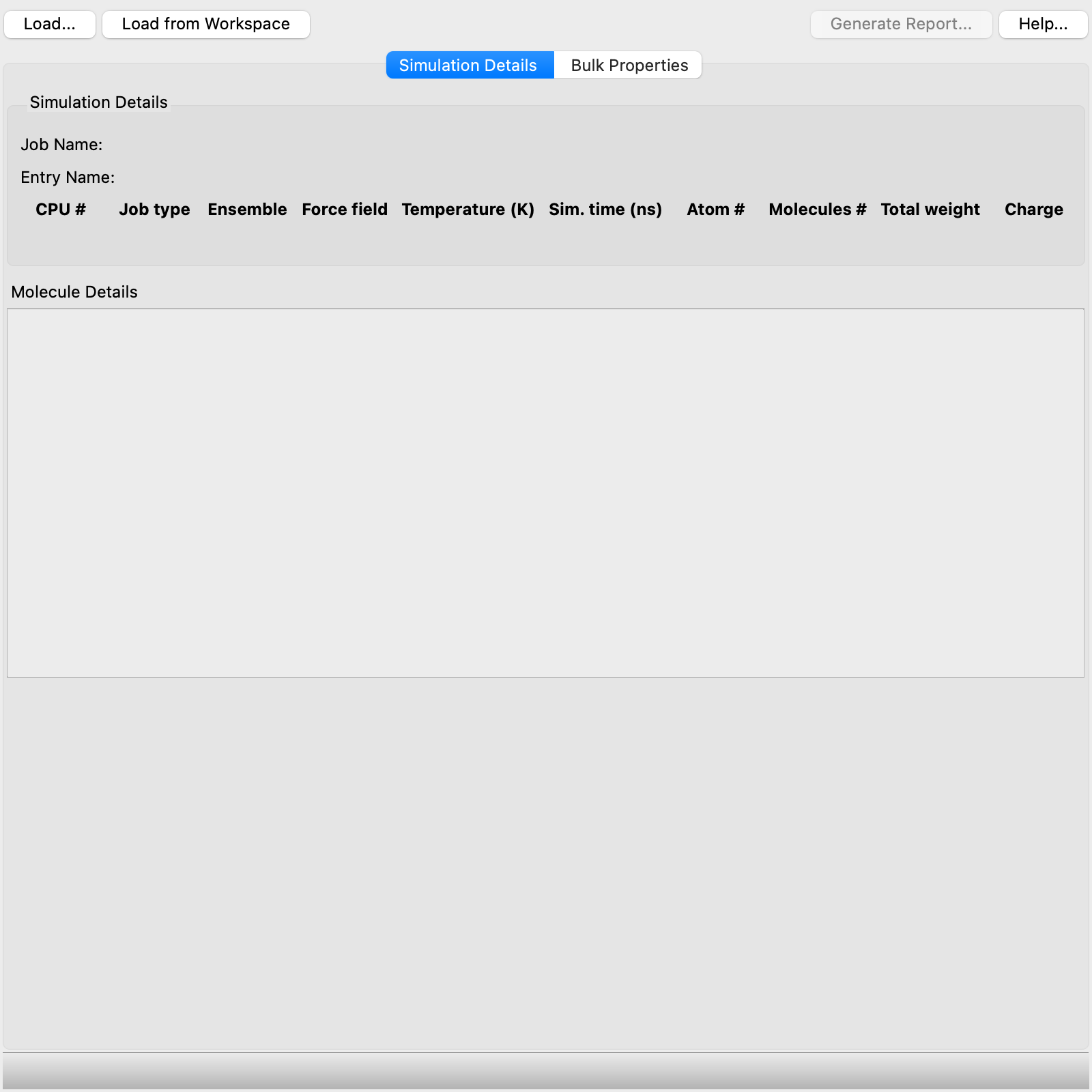
- Simulation Details tab
-
This tab shows data on the simulation. At the top is information on the job that was run, including details of the running of the job and the job input. Below this information is information on each molecule in the simulation, including a SMILES string, molecular formula, and 2D structure, the number of molecules in the simulation box, number of atoms, molecular weight, charge, and number of rotatable bonds.
- Bulk Properties tab
-
In this tab you can display plots of various bulk properties as a function of simulation time.
If you selected the option to calculate the specific heat capacity, the value (Cp or Cv depending on the ensemble) is displayed at the top of the tab. It is displayed for the NPT and NVT ensembles, but not the NVE ensemble.
The range over which the properties are evaluated is displayed at the top right. You can set the range by clicking Set Range, and setting the lower and upper frame limits for the analysis in the dialog box that opens. This is useful for removing the initial equilibration from the analysis so that the average values are for the converged simulation.
There are two plot areas, each of which has the following features:
- Property menu, from which you can choose the bulk property to display on the plot. The items on the menu depend on which properties were generated in the simulation.
- Average and standard deviation of the property computed over the simulation time, displayed above the plot.
- Plot of property as a function of time.
- Bar chart (histogram) showing the distribution of property values during the course of the simulation. There are 10 bins, divided equally over the range of property values.
Upper plot:
There are two related properties that you can plot, the simulation cell volume and the density. If either of these properties is changing significantly, the simulation has not converged. With the OPLS force field (FF), the density of organic and inorganic condensed matter can usually be obtained with an error of less than 3% compared to experiment.
Lower plot:
There are three properties that you can plot:
-
Cohesive energy—The cohesive energy is the energy of the cell divided by the number of molecules in the cell, minus the energy of a single molecule in the gas phase,

-
Solubility parameter—The solubility parameter δ for a pure liquid is defined as

where ΔHv is the heat of vaporization and Vm is the molar volume.
In addition to the solubility parameter, the van der Waals (vdW) and electrostatic contributions to (the square of) this quantity can be selected and plotted. Data on the contributions are added to the report as well.
-
Heat of vaporization—The heat of vaporization is calculated from the energy of the periodic unit cell minus the sum of the N individual molecules, Ei, averaged over the MD trajectory, as
ΔHv = 〈 Ecell − ΣiEi 〉 + RT.
These properties are only available for plotting for neutral systems.