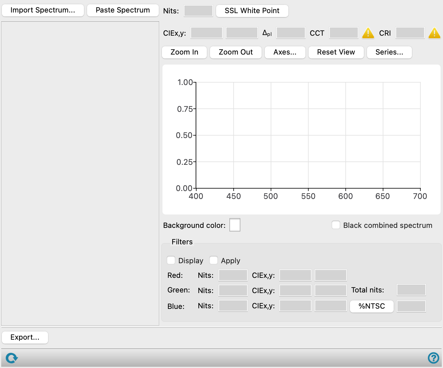
Multispectra Analysis Panel
Combine and adjust visible spectra to generate a spectrum and analyze its color properties.
To open this panel: click the Tasks button and browse to Materials → Tools → Multispectra Analysis.
The following licenses are required to use this panel: MS Maestro
- Using
- Features
- Additional Resources
Using the Multispectra Analysis Panel
This panel can be used to examine how multiple spectra and color filters can be combined in a device to produce lighting or display with desired color characteristics. There are a few main use cases:
-
Spectra of known red, green and blue emitters can be imported into the panel. These spectra can then be added together in the main plot to show what the resulting combined output spectra would look like. The intensity of the individual component spectra can be varied so as to account for cavity effects, device architecture, and relative efficiency.
Color characteristics relevant to lighting and display are calculated for the combined spectrum, such as brightness, CIEx,y coordinates, correlated color temperature, and color rendering index. The change in these color metrics can be explored both as a function of component spectra intensity and by shifting the color of one or more of the component spectra – simulating a chemical modification of the emitter. When a shifted spectrum yields a combined spectrum with better color metrics, you can use the Jaguar TDDFT method and the Calculate Band Shape Panel in conjunction with structure enumeration to explore what chemical modifications of the emitter could bring about the desired shift.
Red, green and blue color filters can be applied to the combined spectrum to simulate the filters on display pixels. Once the filters are applied, the %NTSC color gamut of the resulting three spectra can be examined. The percent transmission of the filters can be modified to simulate changing thickness, and the transmissive range of the filters can be shifted to simulate different filters.
-
Features of the panel can also be used to do analysis of actual device spectra. For instance, the spectrum of a white device can be imported, along with the known spectra of the component emitters. By subtracting the different component spectra from the white emitter, regions of the white spectrum that appear to be missing or enhanced relative to the raw components can be identified. These regions may be due to, among other reasons, cavity effects due to device architecture, quenching effects due to the location of the charge recombination zone, or chemical interactions in the device such as exciplex formation.
If the efficiency (often measured in %EQE – external quantum efficiency) of the emission in the component spectra are known, then the efficiency of the emitters in the device can be estimated by scaling each component spectrum so that subtracting them from the white spectrum cancels it out as closely as possible. This can give indications of emission layers that are performing suboptimally.
-
Comparative analysis can be performed on published spectra. Using the Digitize Curves Panel, spectral data on publications can be digitized and imported into this panel for quantitative analysis by comparison with known emitter spectra.
The spectrum files that are imported are essentially a two-column, tab-separated list of wavelengths in nm and intensities in W sr-1 m-2 (the SI unit of radiance). This is all that is required, so spectra can be exported in tab-separated CSV format, and used in this panel. The columns can optionally be labeled, e.g. with nm and intensity. You can add lines at the top of the file to specify a name for the spectrum (name=text), the external quantum efficiency (eqe=value), and the device (device=text). The device text is not used in the panel, but is added to any exported spectrum. The first few lines of one of the example spectra are given below:
name=Example green
eqe=10
nm	intensity
386.5823	-9.9E-06
393.69797	3E-06
405.58046	0.00004
420.08814	0.0001
For filters, the format is a two-column tab-separated list of wavelengths in nm and transmission, either as a fraction or a percentage. Comment lines may be added, beginning with #.
Multispectra Analysis Panel Features
- Import Spectrum button
-
Import a spectrum to be used in the combination and analysis. Opens a dialog box in which you can locate and import the desired spectrum. Three example red, green, and blue spectra are available in the distribution and are shown by default when you click this button. If the spectrum file does not have a name, you must provide one.
- Paste Spectrum button
-
Paste a spectrum from the clipboard into the panel. The content of the clipboard must have the format of a spectrum file.
- Base spectrum display and tools
-
Each imported or pasted spectrum is shown in a window with the same set of tools, described below.
- spectrum display management buttons
-
These buttons perform display and ordering operations on the spectrum display. They allow for easy duplication and rearrangement of spectrum displays.


Show or hide the contents of the spectrum display. When hidden, only the spectrum display number, label (if any) and these buttons are displayed. This is useful when you have a number of spectrum displays and want to compare two separate spectrum displays, for example. 

Move the spectrum display up or down one place in the list. 
Duplicate the spectrum display. This is useful for creating similar spectrum displays with variations on the settings. 
Delete the spectrum display. - Nits text box
-
Displays the luminance of the spectrum, in candela per square meter (nits). This is the Y value in the CIE xyY color space.
- CIEx,y text boxes
-
Displays the x and y values from the CIE xyY color space for the spectrum.
- %EQE text box
-
Displays the percentage external quantum efficiency value.
- Scale slider
-
Adjust the scale of spectrum intensities. This adjusts the amount of the spectrum in the combined spectrum. The luminance value and the external quantum efficiency are updated to reflect the change, and the value above the slider.
You can use the arrow keys to do fine adjustments of the slider position once the slider is selected.
- Shift slider
-
Shift the maximum of the main spectrum peak to higher or lower wavelengths. This is useful for comparing the shapes of spectra, in combination with the Normalize button to make them the same height in the main plot area.
You can use the arrow keys to do fine adjustments of the slider position once the slider is selected.
- Plot area
-
Displays the spectrum, which fills the vertical height of the plot area.
- Show option
-
Show the spectrum in the combined spectrum plot area. It is removed from this area when you deselect this option.
- Add option
-
Add the spectrum to the combined spectrum. The amount added is controlled by the scale slider. This is useful for building a composite spectrum. When this option is deselected, the addition is undone. Only one of Add or Subtract can be selected at any time.
- Subtract option
-
Subtract the spectrum from the combined spectrum. The amount added is controlled by the scale slider. This is useful for removing components from a spectrum to find unknown components. Negative values resulting from the subtraction are shown as zero. When this option is deselected, the subtraction is undone. Only one of Add or Subtract can be selected at any time.
- Normalize button
-
Normalize the spectrum so that its height is 1.0 in the combined spectrum plot area. This is useful if you are comparing two spectra (in the absence of a combined spectrum): you can shift them to coincide and normalize the heights to compare them.
- Reset button
-
Reset the position and scale of the spectrum to its original values.
- Combined spectrum section
-
This area displays various spectra: the input spectra, when you click Show for a spectrum, a combined spectrum, when you click Add or Subtract for any of the input spectra, and the filter spectra, when you click Show for any of them. Most of the features in this section apply to the combined spectrum.
- Nits text box
-
Displays the luminance of the combined spectrum, in nits.
- SSL White Point button
-
Show the Solid State Lighting white point, as a red dot, on a plot of the CIE xyY color space, in a separate panel. The plot also shows the ANSI standard quadrangles that define the color coordinates for the various official white color temperatures, used as ratings for light bulbs and displays. If the combined spectrum has a color that falls within one of these quadrangles, it is considered to meet the criteria for a white of a particular temperature.
- CIEx,y text box
-
Displays the x and y values from the CIE xyY color space for the combined spectrum.
- Δpl text box
-
Displays the distance from the Planckian locus in the CIE 1960 uv space.
- CCT text box
-
Displays the correlated color temperature. The CCT is only valid if the white point falls within 0.05 of the Planckian locus in CIE 1960 uv space. A green check mark indicates a valid CCT, a red warning sign indicates an invalid CCT.
- CRI text box
-
Displays the CIE color rendering index for the spectrum. THe CRI is only valid if the CIE 1960 uv coordinates of the reflected spectrum is within 0.0054 of the reference, which is the Planckian locus for CCT < 5000, and daylight locus for CCT >= 5000. The check mark or warning sign indicates validity.
- Plot buttons
-
Use these buttons to configure the plot.
- Zoom In—Zoom in on the plot. Each click zooms in by a predefined factor, enlarging the view of the current center of the plot. You can also zoom in on a particular area by dragging out a rectangle.
- Zoom Out—Zoom out by a predefined factor. Each click zooms out by a predefined factor, to show more of the plot.
- Axes—Set the range and labeling options for the axes. Opens the Axes Parameters Dialog Box.
- Reset View—Reset the view of the plot to the original zoom and pan values.
- Series—Set up the appearance of the plot series, such as color, symbol, lines. Opens the Series Parameters Dialog Box.
- Plot area
-
The intensity is plotted against the wavelength in this area. The scale of the Y axis is adjusted with changes in the component spectra so that the combined spectrum fills the vertical space.
You can zoom in to an area by dragging out a rectangle.
- Background color color selector
-
Set the background color of the plot area by clicking on the color square and choosing a color from the Select Color dialog box. This is useful if the color of the combined plot is close to white.
- Black combined spectrum option
-
Plot the combined spectrum in black, rather than with the predicted color.
- Filters section
-
Specify filters for analyzing the combined spectrum.
- Display option
-
Show or hide the filter spectra section on the right side of the panel.
- Apply option
-
Apply the filters to the combined spectrum, to generate three spectra which are the product of the combined spectrum with each filter.
- Red/Green/Blue spectral data text boxes
-
These text boxes display the luminance (Y, in nits) and x and y values from the CIE xyY color space for the combined spectrum filtered by each of the filters.
- Total nits text box
-
Displays the total luminance in nits.
- %NTSC button and text box
-
Show the percentage of the CIE color space covered by the current filtered spectrum compared to the NTSC color gamut. The button opens the Color Gamut dialog box, where the NTSC gamut and the filtered spectrum gamut are shown on the full CIE xyY color space. The corners of the triangle are the CIE x, y coordinates of the filtered spectra. The text box shows the percentage.
- Filter spectra section
-
The spectra of the filters are displayed in this section. Each has the same set of features, described below.
- Color filter text box
-
Shows the name of the filter file for the particular color.
- Show option
-
Show the filter spectrum in the combined spectrum plot area.
- Scale slider
-
Adjust the scale of the filter spectrum transmission.
You can use the arrow keys to do fine adjustments of the slider position once the slider is selected.
- Shift slider
-
Shift the maximum of the main spectrum peak to higher or lower wavelengths.
You can use the arrow keys to do fine adjustments of the slider position once the slider is selected.
- Plot area
-
Displays the filter spectrum.
- New Filter button
-
Replace the filter with a new filter from file. Opens a file selector to choose the filter file; the name is displayed in the Color filter text box.
- Reset button
-
Reset any changes made to the spectrum (scale, shift).
- Export button
-
Export the spectral data or images to files. Opens the Export Spectra dialog box, in which you can choose to export data or images, select the spectrum or the chart to export, and supply additional information. Clicking OK opens a file browser to find a location and name the file.
- Status bar
-
 to reset the panel to its default settings and clear any data from the panel.
If you can submit a job from the panel, the status bar displays information about the current job settings and status for the panel. The settings include the job name, task name and task settings (if any), number of subjobs (if any) and the host name and job incorporation setting. The job status can include messages about job start, job completion and incorporation.
The status bar also contains the Help button
 , which opens an option menu with choices to open the help topic for the panel (Documentation), launch Maestro Assistant, or if available, choose from an option menu of Tutorials. If the panel is used by one or more tutorials, hover over the Tutorials option to display a list of tutorials. Choosing a tutorial opens the tutorial topic.