An Overview of Multi-Property Optimization (MPO)
In materials design, it is often necessary to consider multiple properties when forming a desired property profile for a compound. Multi-property optimization (MPO) can be used to capture the complexity of this problem by quantifying how well the properties of a compound matches an ideal set of desired properties with a single numeric value: the MPO score.
The MPO Process
- Choose a set of desired properties that you want to include in the multi-property optimization.
- For each property, determine the optimization method, cutoff criterion, and weight. The optimization method and the cutoff criterion serve to identify some target value for the property. These are discussed in detail in the following sections. A set of properties with defined cutoffs is known as a multi-property profile (MPP).
- Calculate the value of each property in the MPP for a compound.
- An individual property score, which ranges from 0 (worst) to 1 (best) is assigned to each property based on how close the calculated property value is to the desired property value as defined by the optimization method and the cutoff criterion.
- The MPO score for a compound, which ranges from 0 (worst) to 1 (best), is obtained by taking the weighted geometric mean of the individual property scores for that compound. The weights of each individual property are the ones defined in step 2. The closer a compound's MPO score is to 1, the closer that compound is to having the desired property profile.
Scoring an Individual Property
The calculated value of a property is mapped to a normalized score between 0 and 1 with the use of a logistic curve (or Fermi function):

This is done so that all properties are on the same scale. The logistic curve is determined from two threshold values (a and b) that divide the property range into "good" values, "ok" values, and "bad" values. These threshold values define the shape of the logistic curve, as they are set to be at the inflection points of the curve. For each property, the user defines an optimization method for how the optimal property value is reached: Maximize, Minimize, and Targeted value. The three optimization methods need various criterion to determine “good”, “ok” and “bad” value ranges:
Maximize
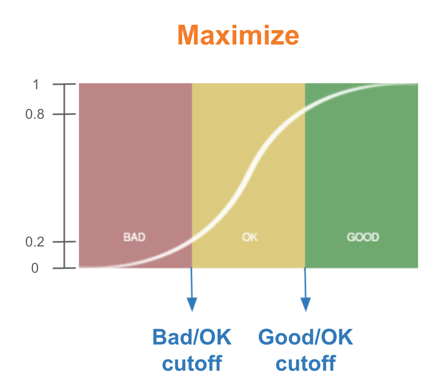
For the Maximize optimization method, the higher the property value the better. The higher property value (x-axis), the closer to 1 the individual property score (y-axis).
The user defines a Bad/OK cutoff and a Good/Ok cutoff as x values in the units of the property. The values for y=f(x) are set to the inflection points of the logistic curve: y=0.2 at the Bad/OK cutoff and y=0.8 at the Good/OK cutoff.
For example, a user chooses to use the Maximize optimization method for Property A in the MPO. The Bad/OK cutoff is defined to be 20 and the Good/OK cutoff is defined to be 50. If the calculated value of Property A for a compound turns out to be 30, then the individual property score is somewhere between 0.2 and 0.8. The compound has an "ok" value for Property A.
Minimize
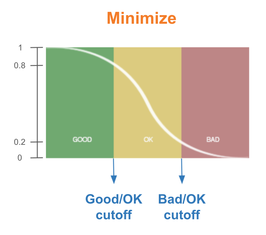
For the Minimize optimization method, the lower the property value the better. The lower the property value (x-axis), the closer to 1 the individual property score (y-axis).
The user defines a Good/OK cutoff and a Bad/Ok cutoff as x values in the units of the property. The values for y=f(x) are set to the inflection points of the logistic curve: y=0.8 at the Good/OK cutoff and y=0.2 at the Bad/OK cutoff.
For example, a user chooses to use the Minimize optimization method for Property B in the MPO. The Good/OK cutoff is defined to be 5 and the Bad/OK cutoff is defined to be 10. If the calculated value of Property B for a compound turns out to be 12, then the individual property score will be less than 0.2. The compound has an "bad" value for Property B.
Targeted
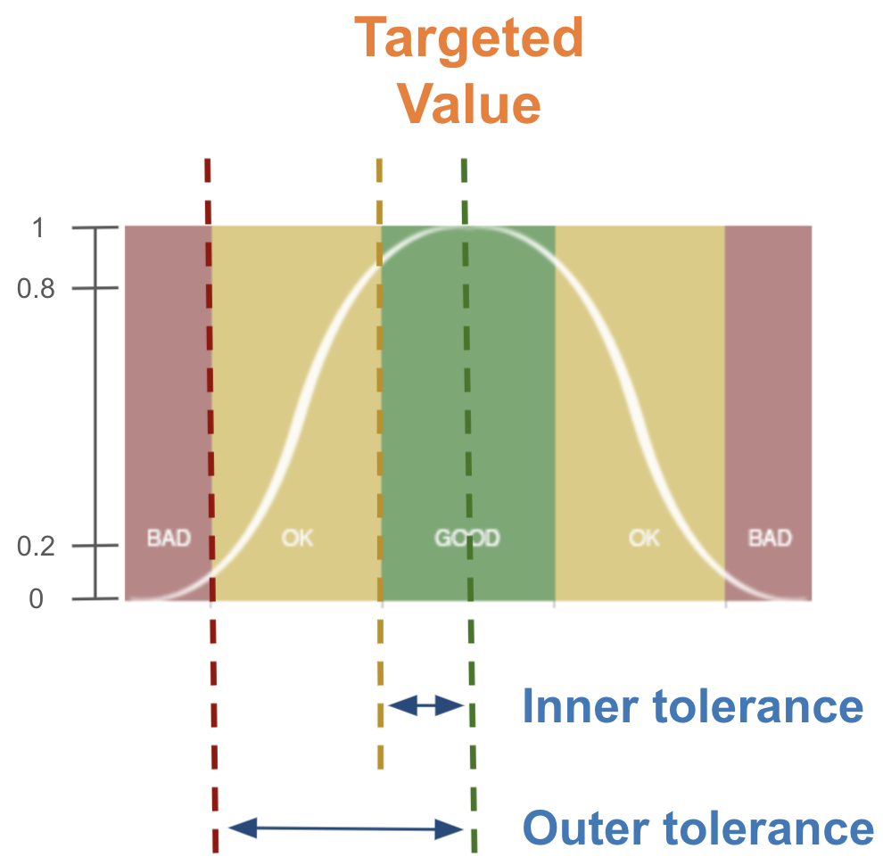
For the Targeted optimization method, the user sets a desired value for the property. At this desired value, the individual property score (y-axis) is 1. The further away from the targeted value, the lower the score. Two logistic curves are required on either side of the user defined Targeted value. In addition, the user defines an Inner tolerance and an Outer tolerance. The smaller the tolerance, the steeper the curve.
The inner tolerance is the range where the property value is still "good". If the absolute difference between the targeted value and the property value is within the inner tolerance, the property value is still in the “good” range. The inner tolerance thus defines the Good/OK cutoff on either side of the targeted value.
The outer tolerance is the range where the property value is still "good" or "ok". If the absolute difference between the targeted value and the property value is within the outer tolerance, the property is in the “ok” range if the property value is outside the inner tolerance and the “good” range if the property value is inside the inner tolerance. The outer tolerance thus defines the Bad/OK cutoff on either side of the targeted value.
For example, a user chooses to use the Targeted optimization method for Property C in the MPO. The Targeted value is set to be 100. The Inner tolerance is set to be 10 and the Outer tolerance is set to be 30. If the calculated value of Property C for a compound turns out to be 95, this value is within the Inner tolerance and the individual property score will be between 0.8 and 1. The compound has a "good" value for Property C. This would also be the case if Property C had a value of 105.
MPO Scores
The MPO score is obtained by taking the weighted geometric mean of the individual property scores in the MPP:

The scores range from 0(worst) to 1(best). The geometric mean is used rather than the arithmetic mean to ensure that one bad value is not underrepresented in the MPO score. The weight for each property is user defined. If the weight for all properties in the MPO score calculation is equal to one another, the properties are weighted equally.