Machine Learning Property Prediction Panel
Use pre-built machine learning models to make predictions on various properties.
To open this panel: click the Tasks button and browse to Materials → Informatics → Machine Learning Property Prediction.
The following licenses are required to use this panel: MS Maestro, MS Informatics
- Using
- Features
- Additional Resources
Using the Machine Learning Property Prediction Panel
The Machine Learning Property Prediction panel utilizes pre-built machine learning (ML) models to make predictions of various properties for polymers, organic compounds, and organometallic complexes. The available ML models, and the properties they predict are listed below:
| Machine Learning Model | Properties | Required Input System | References for Training Data | ||||
| Density of molecular liquids | The density (g cm-3) of organic molecules in the liquid phase at 293.15 K and 1 atm | organic molecule | 67 | ||||
| Polymer dielectric constant | Relative dielectric permittivity (Dk) of polymers | monomer unit | 69 | ||||
| Polymer dissipation loss | Predicts the dissipation loss (Df) of polymers | monomer unit | 69 | ||||
| Polymer glass transition temperature | Glass transition temperature (Tg) of polymers (in Kelvin) | monomer unit | 69, 70 | ||||
| Viscosity of organic liquids | Viscosity of organic molecules in the liquid phase (in cP) | organic molecule | 57 | ||||
| Volatility for organic molecules | Boiling/sublimation point (in Kelvin) and vapor pressure (in Torr) | organic molecule | 71 | ||||
| Volatility for organometallic molecules | Boiling/sublimation point (in Kelvin) | organometallic or inorganic molecule | 71 | ||||
| Optoelectronic properties of molecules | Various optoelectronic properties for organic molecules in solution or as thin films: absorption peak position, absorption bandwidth, extinction coefficient, emission peak position, emission bandwidth, emission lifetime, photoluminescence quantum yield | organic molecule | 68 | ||||
| Oxidation potential | Oxidation potential (in V) in acetonitrile solvent at 298 K, referenced to SCE | organic molecule | Learn More | ||||
| Reduction potential | Reduction potential (in V) in acetonitrile solvent at 298 K, referenced to SCE | organic molecule | Learn More | ||||
| Aqueous solubility | Aqueous solubility of small molecules (in log10(mol/L)) | organic molecule | 65, 66 | ||||
| Non-aqueous solubility | Non-aqueous solubility of small molecules (in log10(mol fraction)) | organic molecule | 83 | ||||
| Singlet-triplet energy gap | Vertical singlet -triplet energy gap ΔES1T1 (in eV) in toluene solvent | organic molecule | Learn More | ||||
| Melting point | Melting point (in Kelvin) of small organic molecules | organic molecule | 84 | ||||
| Scaled HOMO | Energy of the HOMO (in eV) in toluene solvent | organic or organometallic molecule | Learn More | ||||
| Scaled LUMO | Energy of the LUMO (in eV) in toluene solvent | organic or organometallic molecule | Learn More | ||||
| Triplet Energy (E(S0T1)) | Energy gap for the ground singlet state (S0) and lowest triplet state (T1) (in eV) in toluene solvent | organic or organometallic molecule | Learn More | ||||
| Hole reorganization energy | Hole reorganization energy (in eV) in toluene solvent | organic molecule | Learn More | ||||
| Electron reorganization energy | Electron reorganization energy (in eV) in toluene solvent | organic molecule | Learn More | ||||
| Triplet Reorganization Energy | Triplet reorganization energy (in eV) in toluene solvent | organic molecule | Learn More |
All ML models available in this panel were trained with Schrödinger's automated ML workflow, DeepAutoQSAR.
The ML models used to predict Tg, Dk, and Df represent polymers as monomer units with connection points denoted as two At atoms:
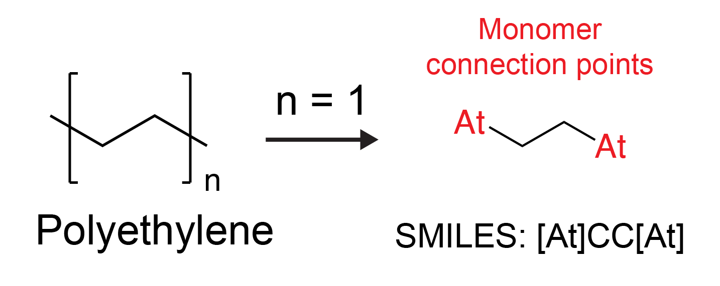
When using these models, the input system must be a monomer with At atoms at the connection points. Alternatively, you can use the Mark Monomer Head and Tail Panel to prepare a monomer for property prediction.
The general workflow of the panel is:
-
Review information on a model from the Model Performance section to ensure you are using the appropriate model.
-
If predicting Tg, Dk, or Df, prepare monomer units as explained above and select. If predicting volatility, select either organic molecules or organometallic complexes depending on the model that you are using. If predicting any other properties, select the molecules of interest appropriately.
-
Choose whether to predict in Interactive mode or Batch mode. If Interactive mode is selected, predictions are made in the Results table within the panel, and up to 10 entries can be selected. If Batch mode is selected, a new entry group is incorporated after the job is completed, and the predicted properties can be viewed from the Project Table.
-
Choose the machine learning model and input any additional prediction parameters (e.g., frequency for Dk or Df).
-
Use the Predict button to make property predictions in Interactive mode, or use the Job toolbar to make predictions in Batch mode.
To write out the input file and a script for running the job from the command line, click the arrow next to the Settings button  and choose Write.
Machine Learning Property Prediction Panel Features
- Use structures from option menu
- Interactive mode option
- Batch mode option
- Machine learning model option menu
- Density of molecular liquids
- Polymer dielectric constant
- Polymer dissipation loss
- Polymer glass transition temperature
- Viscosity of organic liquids
- Volatility for organic molecules
- Volatility for organometallic molecules
- Optoelectronic properties of molecules
- Oxidation potential
- Reduction potential
- Aqueous solubility
- Non-aqueous solubility
- Singlet-triplet energy gap
- Melting point
- Scaled HOMO
- Scaled LUMO
- Triplet Energy (E(S0T1))
- Hole reorganization energy
- Electron reorganization energy
- Triplet reorganization energy
- Download Model button
- Model available text
- Model Information section
- Results from selected entries section
- Job toolbar
- Status bar
- Use structures from option menu
-
Choose the structure source for property prediction.
- Project Table (n selected entries)—Use the entries that are currently selected in the Project Table or Entry List. The number of entries selected is shown on the menu item.
- Project Table (n selected entries)—Use the entries that are currently selected in the Project Table or Entry List. The number of entries selected is shown on the menu item.
- Interactive mode option
-
Predict properties for the selected entries in the Project Table or Entry List and display them immediately in the panel. Click the Predict button to list predictions in the Results table. Predictions can only be made for up to 10 selected entries. The predicted properties and prediction uncertainties can be viewed from the Project Table. The Project Table column headers associated with the predicted properties are listed under the Batch mode option. If you want to make predictions for more than 10 entries, use Batch mode instead.
- Batch mode option
-
Predict properties for the selected entries in the Project Table or Entry List. Use the Job toolbar to run the job. A new entry group is incorporated after the job is completed with structures corresponding to successful predictions, and the predicted properties and prediction uncertainties can be viewed from the Project Table. The Project Table column headers associated with the predicted properties are:
- Density (g/cm3) at n—Density of molecular liquids selected as the ML model
- Polymer Dk at n—Polymer dielectric constant selected as the ML model
- Polymer Df at n—Polymer dissipation loss selected as the ML model
- Polymer Tg (K)—Polymer glass transition temperature selected as the ML model
- Viscosity at n—Viscosity of organic liquids selected as the ML model
- Evaporation temperature (K) at n—Boiling point selected as the prediction property using the Volatility for organic molecules or Volatility for organometallic molecules ML models.
- Vapor pressure (Torr) at n—Vapor pressure selected as the prediction property using the Volatility for organic molecules ML model
- Oxidation Potential (V)—Oxidation potential selected as the ML model
- Reduction Potential (V)—Reduction potential selected as the ML model
- Aqueous Solubility (log mol/L)—Aqueous solubility selected as the ML model
- NonAq Solubility (log mol frac) at n—Non-aqueous solubility selected as the ML model
- Singlet Triplet Energy Gap (eV)—Singlet-triplet energy gap selected as the ML model
- Melting Point (K)—Melting point selected as the ML model
- Scaled HOMO Energy (eV)—Scaled HOMO selected as the ML model
- Scaled LUMO Energy (eV)—Scaled LUMO selected as the ML model
- Triplet Energy (eV)—Triplet Energy (E(S0T1)) selected as the ML model
- Hole Reorganization (eV)—Hole reorganization energy selected as the ML model
- Electron Reorganization (eV)—Electron reorganization energy selected as the ML model
- Triplet Reorganization Energy (eV)—Triplet reorganization energy selected as the ML model
where n is the specified prediction parameter with the selected unit. Go to Materials Science to add a column to the Project Table. See the Optoelectronic properties of molecules ML model description for Project Table column headers for optoelectronic properties.
- Machine learning model option menu
-
Select which machine learning model to use for the prediction of properties. The choice of model determines what properties can be predicted. Some machine learning models require additional parameters beyond the input structures.
- Density of molecular liquids
-
This model predicts the density of small organic molecules in the liquid phase at 293.15 K and 1 atm in g cm-3.
- Polymer dielectric constant
-
This model predicts the relative dielectric permittivity (Dk) of polymers at a specified frequency.
- Polymer dissipation loss
-
This model predicts the dissipation loss (Df) of polymers at a specified frequency.
- Polymer glass transition temperature
-
This model predicts the glass transition temperature (Tg) of polymers in Kelvin.
- Viscosity of organic liquids
-
This model predicts boiling/sublimation point in Kelvin and vapor pressure in Torr of organic molecules. You can also plot the boiling/sublimation point over a range of pressures in Interactive mode.
- Property option menu
-
Choose a property to predict using the selected model, from Boiling point and Vapor pressure.
- Predict at options
-
- Boiling point is selected from the Property option menu
-
Select at from the option menu to predict the boiling/sublimation point at a given pressure. Specify the pressure in the text box, and select the unit for the pressure from Torr, bar, atm. The boiling/sublimation point is given in Kelvin (K). The accepted range is 10-2 to 22800 torr for organic molecules and 10-10.
Select every from the option menu to instead predict the boiling/sublimation point at pressure intervals. Specify an interval of pressure at which to predict the boiling/sublimation point in the text box. , the unit for the pressure from the option menu, and the range of pressure in the from and to text boxes. After clicking the Predict button, a plot is shown in the Results from selected entries section which displays the boiling/sublimation point at the range of specified pressures as a line graph. The accepted range is 10-2 to 22800 torr for organic molecules. The every option is only available in Interactive mode.
- Vapor pressure is selected from the Property option menu
-
Specify the temperature at which to predict the vapor pressure in the text box, and select the unit for the temperature either in Kelvin or degree Celsius. The vapor pressure is given in Torr. The accepted range is 68K to 723K.
-
This model predicts various optoelectronic properties of organic molecules in solution or as thin films. The Property option menu lists all of the properties available for prediction.
The resulting entry title contains thin film if the Thin film option was selected or the solvent name if the Solution in option was selected.
Some, but not all, experimental data on which the model was trained was taken at room temperature. See Ref 68 for more information.
- Property option menu
-
Choose a property to predict using the selected model:
- Absorption peak position—This model predicts the wavelength in the visible region for which the absorption spectrum has the highest intensity in nm. The associated Project Table column header is Absorption Lmax (nm).
- Absorption bandwidth—This model predicts the bandwidth of the Absorption peak position in full width at half maximum (FWHM) in cm-1. The associated Project Table column header is Absorption Bandwidth (cm-1).
- Extinction coefficient—This model predicts the molar extinction coefficient in log(mol-1dm3cm-1). The associated Project Table column header is Extinction Coefficient (log mol-1dm3cm-1).
- Emission peak position—This model predicts the wavelength of the fluorescence maximum in nm. The associated Project Table column header is Emission Emax (nm).
- Emission bandwidth—This model predicts the bandwidth of the Emission peak position in full width at half maximum (FWHM) in cm-1. The associated Project Table column header is Emission Bandwidth (cm-1).
- Emission lifetime—This model predicts the fluorescence or excited state lifetime in log10(ns). The associated Project Table column header is Emission Lifetime (log ns).
- Photoluminescence quantum yield—This model predicts the photoluminescence quantum yield (PLQY), the ratio of photons emitted to photons absorbed, for organic molecules. The associated Project Table column header is Photoluminescence Quantum Yield.
- Thin film option
-
Calculate the prediction property for the structures as a thin film.
- Solution in option and menu
-
Calculate the prediction property for the structures of interest in solution with the solvent selected from the menu.
- Oxidation potential
-
This model predicts the oxidation potential (in V) of organic molecules in acetonitrile solvent at 298 K. All values are referenced to the saturated calomel electrode (SCE).
-
Models were generated by the Schrödinger QM-ML approach detailed in QM-Based Machine Learning Models. The model was initially trained on 200,000 chemically diverse molecules generated internally using quantum mechanics (QM) calculations. Then, to improve performance, this initial model was fine-tuned using a smaller set of 400 experimental values.
- Reduction potential
-
This model predicts the reduction potential (in V) of organic molecules in acetonitrile solvent at 298 K. All values are referenced to the saturated calomel electrode (SCE).
-
Models were generated by the Schrödinger QM-ML approach detailed in QM-Based Machine Learning Models. The model was initially trained on 170,000 chemically diverse molecules generated internally using quantum mechanics (QM) calculations. Then, to improve performance, this initial model was fine-tuned using a smaller set of 200 experimental values.
- Aqueous solubility
-
This model predicts the aqueous solubility of small organic molecules in log10(mol/L).
- Non-aqueous solubility
-
This model predicts the non-aqueous solubility of small organic molecules in a specified solvent and at a specified temperature in log10(mol fraction). The resulting entry title contains the solvent name.
- Predict at options
-
Specify the temperature at which to predict the non-aqueous solubility in the text box, and select the unit for frequency from Kelvin or Celsius in the option menu. The suggested range is 243.15 to 403.15 K.
- Solution in option menu
-
Calculate the non-aqueous solubility for the structures of interest in the solvent selected from the menu.
This model predicts the vertical singlet -triplet energy gap, ΔES1T1 in eV.
Models were generated by the Schrödinger QM-ML approach detailed in QM-Based Machine Learning Models. The model was trained using a library of approximately 55,000 organic compounds with chemistry typically found in OLED device materials. Property values were computed using quantum mechanics (QM) calculations.
This model predicts the melting point of small organic molecules in Kelvin.
This model predicts the energy level for the highest occupied molecular orbital (HOMO) for molecules in eV, which is taken as the change in the adiabatic Gibbs free energy for the loss of a single electron in toluene: 
Models were generated by the Schrödinger QM-ML approach detailed in QM-Based Machine Learning Models. The model was trained using a library of approximately 55,000 organic compounds and 4,500 organometallic complexes (containing Ir or Pt) with chemistry typically found in OLED device materials. Property values were computed using quantum mechanics (QM) calculations.
This model predicts the energy level for the lowest unoccupied molecular orbital (LUMO) for molecules in eV, which is taken as the change in the adiabatic Gibbs free energy for the gain of a single electron in toluene: 
Models were generated by the Schrödinger QM-ML approach detailed in QM-Based Machine Learning Models. The model was trained using a library of approximately 55,000 organic compounds and 4,500 organometallic complexes (containing Ir or Pt) with chemistry typically found in OLED device materials. Property values were computed using quantum mechanics (QM) calculations.
This model predicts the energy difference between the lowest triplet state (T1) and the ground singlet state (S0) of a molecule in eV, which is taken as the change in the adiabatic Gibbs free energy for the S0→T1 transition in toluene.
Models were generated by the Schrödinger QM-ML approach detailed in QM-Based Machine Learning Models. The model was trained using a library of approximately 55,000 organic compounds and 4,500 organometallic complexes (containing Ir or Pt) with chemistry typically found in OLED device materials. Property values were computed using quantum mechanics (QM) calculations.
This model predicts the total internal reorganization energy (in eV) for electron transfer between two molecules of the same species: one neutral ( ) and one positively charged (
 ). This energy corresponds to the migration of the positive charge:
  . This energy corresponds to the sum of energies required to relax the geometry of
  undergoing oxidation and
  undergoing reduction. External reorganization of the environment is not considered here.
Models were generated by the Schrödinger QM-ML approach detailed in QM-Based Machine Learning Models. The model was trained using a library of approximately 55,000 organic compounds with chemistry typically found in OLED device materials. Property values were computed using quantum mechanics (QM) calculations.
This model predicts the total internal reorganization energy for electron transfer between two molecules of the same species, one neutral ( ) and one charged (
 ). This energy corresponds to migration of the negative charge:
  . This energy corresponds to the sum of energies required to relax the geometry of
  undergoing reduction and
  undergoing oxidation. External reorganization of the environment is not considered here.
Models were generated by the Schrödinger QM-ML approach detailed in QM-Based Machine Learning Models. The model was trained using a library of approximately 55,000 organic compounds with chemistry typically found in OLED device materials. Property values were computed using quantum mechanics (QM) calculations.
This model predicts the total internal reorganization energy for two molecules of the same species, one in the ground singlet state ( ) and one in the ground triplet state (
 ). This energy corresponds to the sum of energies required to relax the geometry of
  undergoing a
  transition and
  undergoing a
  transition. External reorganization of the environment is not considered here.
Models were generated by the Schrödinger QM-ML approach detailed in QM-Based Machine Learning Models. The model was trained using a library of approximately 55,000 organic compounds with chemistry typically found in OLED device materials. Property values were computed using quantum mechanics (QM) calculations.
When you click this button, an ensemble model for the selected ML model with prediction uncertainty (computed by the standard deviation of individual model predictions) is downloaded. Due to the large file size of the model, it is not available with your Schrödinger software installation and must be downloaded using this button. The download may take up to a few minutes and is complete when Model available is displayed in place of the button. The downloaded ensemble models are used for predictions.
The ensemble models were trained with Schrödinger's automated ML workflow, DeepAutoQSAR. For more information on DeepAutoQSAR, please see the following whitepaper.
The ML model for each optoelectronic prediction property must be downloaded separately.
Displays Model available when the ensemble ML model is downloaded and available for use. Click the Download Model button to initiate the download.
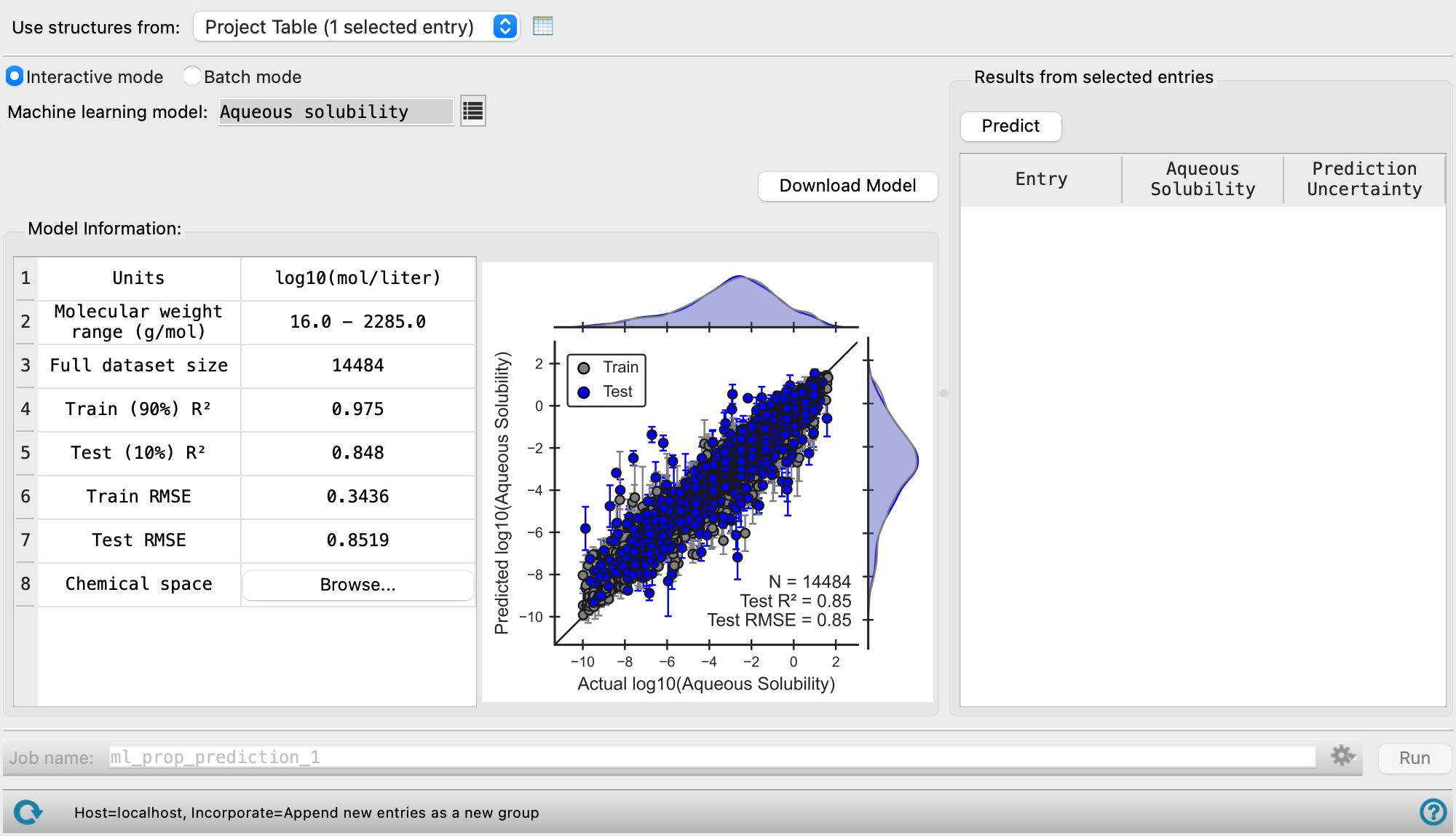
Displays information about the machine learning model used for property prediction. You can use the R2 and RMSE values as well as the ranges shown in the plot to inform how the model performs against experimental values and expected error ranges. Compare the chemical space of the model to your system to determine whether the model is appropriate for your system.
- Model Info Table
-
- Units—The unit of prediction for the ML model.
- Molecular weight range (g/mol)—The molecular weight limits for the ML model. Use of molecules with weights that fall outside of the range may lead to erroneous predictions and is not recommended.
- Full data set size—Total size of the data used to generate the ML model. The data is split into a training set (90% of the training data) and a test set (10% of the training data).
- Training (90%) R2— R-squared value (coefficient of determination) for the training set. The scatter plot used to determine this value is displayed to the right of the Model Info Table.
- Test (10%) R2—R-squared value (coefficient of determination) for the test set. The scatter plot used to determine this value is displayed to the right of the Model Info Table.
- Train RMSE—Root-mean-square error of the training set.
- Test RMSE—Root-mean-square error of the test set.
- Chemical Space—Click the Browse button to open the Chemical space dialog box to visualize the elements covered in the machine learning model in a periodic table. Use of structures containing elements other than those listed may lead to erroneous predictions and is not recommended.
The oxidation and reduction potential models use two datasets for model generation: a large QM-calculated set and smaller experimental set. These models are designed to reproduce the values of QM and experiment holdout sets with minimal error in order maximize chemical coverage without loss of accuracy. Model information is provided for both the QM set and the experimental set in the Model Info Table as (QM) and (Expt), respectively. Model performance and parity plots for both holdout sets are discussed here QM-Based Machine Learning Models.
- Model Performance Plot
-
Displays a parity plot of the predicted value given by the ML model against the actual value (experimental or from QM calculations) for both the training and test set. The distribution of data points within the training and test sets is illustrated along the axes of each parity plot. Additionally, the test set performance metrics along with the total size of the dataset are displayed in the bottom righthand corner of the plot.
Use this section to make immediate predictions for selected entries, up to 10 entries. This section is only available when Interactive mode is selected.
- Predict button
-
Click to populate the section with the prediction of the selected property for the selected entries.
- Results table
-
Displays the Entry name of the selected entries, the value of the predicted property, and the Prediction Uncertainty.
- Boiling/Sublimation Point Plot
-
Displays the boiling/sublimation point in Kelvin at the range of specified pressures as a line graph. The toolbar at the top of the plot has tools for manipulating the plot and for saving images. The buttons that are common to all plot toolbars are described in the Plot Toolbar topic. The plot is only present if Volatility for organic molecules is selected as the Machine learning model, and Boiling point and every are chosen from the Predict options.
Manage job submission and settings. See Job Toolbar for a description of this toolbar.
Only available if Batch mode is selected.
The Job Settings button opens the Machine Learning Property Prediction - Job Settings Dialog Box, where you can make settings for running the job.
 to reset the panel to its default settings and clear any data from the panel.
If you can submit a job from the panel, the status bar displays information about the current job settings and status for the panel. The settings include the job name, task name and task settings (if any), number of subjobs (if any) and the host name and job incorporation setting. The job status can include messages about job start, job completion and incorporation.
The status bar also contains the Help button  , which opens an option menu with choices to open the help topic for the panel (Documentation), launch Maestro Assistant, or if available, choose from an option menu of Tutorials. If the panel is used by one or more tutorials, hover over the Tutorials option to display a list of tutorials. Choosing a tutorial opens the tutorial topic.