OLED Device Machine Learning Panel
Build and apply machine learning models for predicting OLED device properties.
To display this panel: click the Tasks button and browse to Materials → Informatics → OLED Device Machine Learning
The following licenses are required to use this panel: MS Maestro, MS Layered Device ML, MS Informatics (optional)
- Using
- Features
- Additional Resources
Using the OLED Device Machine Learning Panel
The OLED Device Machine Learning Panel can be used to build and apply machine learning (ML) models to predict properties for organic light-emitting diode (OLED) devices. OLED devices are defined as multilayer structures where each layer has a specific material composition and serves a specific purpose. Common types of layers and interfaces in OLED devices are as follow:
-
Anode—The anode serves as the positive electrode in an OLED. It is typically made of a transparent conductive material, such as indium tin oxide (ITO), which allows light from the emissive layer to escape while facilitating the injection of holes into the device layers.
-
Hole Injection Layer (HIL)—This layer is positioned directly above the anode. The HIL facilitates efficient injection of holes into the neighboring hole transport layer (HTL).
-
Hole Transport Layer (HTL)—This layer transports holes from the HIL toward the emissive layer.
-
Electron Blocking Layer (EBL)—Positioned between the HTL and EML, the EBL blocks electrons from leaking into the HTL, further promoting recombination within the EML.
-
Emissive Layer (EML)—The core layer where electrons and holes recombine to form excitons. The EML contains the emitter (fluorescent, phosphorescent, or TADF molecules) often dispersed in a host matrix. The choice of host and dopant affects color purity, efficiency, exciton dynamics, and device stability.
-
Hole Blocking Layer (HBL)—Positioned between the EML and ETL, this layer prevents holes from leaking into the ETL, helping to confine excitons in the emission zone.
-
Electron Transport Layer (ETL)—This layer assists in the movement of electrons from the cathode towards the EML.
-
Electron Injection Layer (EIL)—Located adjacent to the cathode, the EIL improves electron injection by modifying the interface between the cathode and ETL, lowering the barrier for electron transfer.
-
Cathode—The cathode serves as the negative electrode in an OLED. Typically composed of a metal with a low work function (e.g., aluminum, magnesium, or calcium), it efficiently injects electrons into the adjacent layer.
Alternative to traditional experimental methods and physics-based simulations, machine learning models from this panel can be used as a data-driven approach to determining OLED device properties.
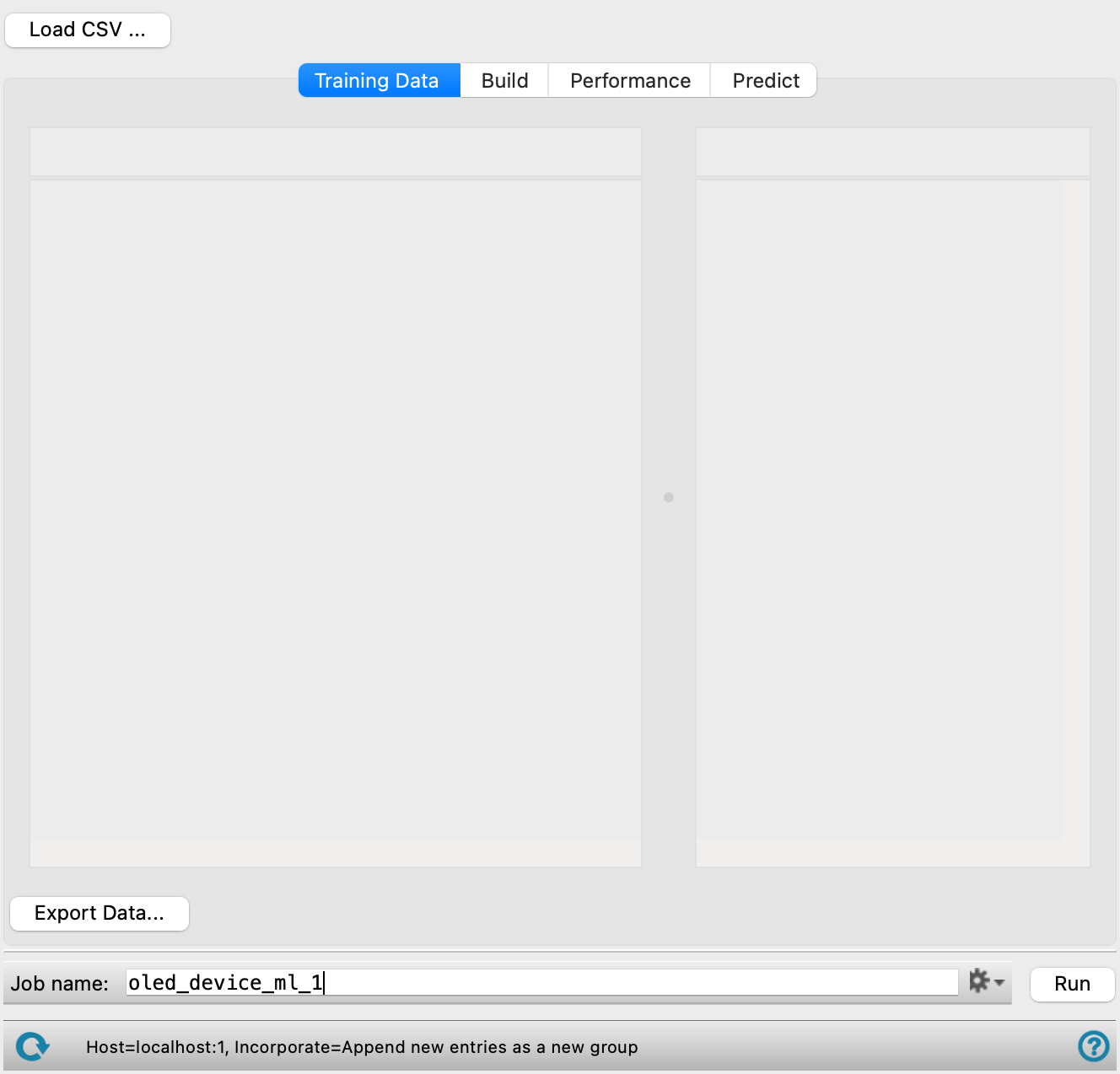
The four tabs in the panel, Training Data, Build, Performance, and Predict, enable a complete ML workflow in one tool:
-
Training Data—Load, view, edit, and plot input device architectures for training a ML models.
-
Build—Specify parameters for training ML models and the properties to be predicted.
-
Performance—Analyze the quality of trained models.
-
Predict—Make predictions for OLED device parameters using a trained ML model from this panel.
The input for this panel is a CSV file containing structural and composition information about the OLED devices and properties of interest. OLED device datasets can be generated by extracting literature data, performing experiments, performing physics-based simulations, or employing predictions from molecule-property models. OLED devices can additionally be designed and visualized in the Optoelectronic Device Designer Panel.The OLED Device Machine Learning panel does not interact with the workspace or Project Table.
The CSV file(s) must contain a specific set of headers to be compatible with the panel.
Each row in the input .csv file is an OLED device with different specifications. Device architectures are defined by layer types, thicknesses, and material composition. The device must be composed of the layer types described in the Using section.
Anode_0_SMILES_0,Anode_0_comp_0,Anode_0_thickness,HIL_0_SMILES_0,HIL_0_comp_0,HIL_0_SMILES_1,HIL_0_comp_1,HIL_0_thickness,HTL_0_SMILES_0,HTL_0_comp_0,HTL_0_thickness,HTL_1_SMILES_0,HTL_1_comp_0,HTL_1_thickness,EBL_0_SMILES_0,EBL_0_comp_0,EBL_0_thickness,EBL_1_SMILES_0,EBL_1_comp_0,EBL_1_thickness,Host_0_SMILES_0,Host_0_comp_0,Host_0_SMILES_1,Host_0_comp_1,Host_0_thickness,Emitter_0_SMILES_0,Emitter_0_wt%_0,Emitter_0_SMILES_1,Emitter_0_wt%_1,HBL_0_SMILES_0,HBL_0_comp_0,HBL_0_thickness,HBL_1_SMILES_0,HBL_1_comp_0,HBL_1_thickness,ETL_0_SMILES_0,ETL_0_comp_0,ETL_0_thickness,ETL_1_SMILES_0,ETL_1_comp_0,ETL_1_thickness,EIL_0_SMILES_0,EIL_0_comp_0,EIL_0_thickness,Cathode_0_SMILES_0,Cathode_0_comp_0,Cathode_0_thickness,num_layers,EQE[%]_max,Lambda(EL)[nm]_max
O=[Sn].O=[In]O[In]=O.O=[In]O[In]=O.O=[In]O[In]=O.O=[In]O[In]=O.O=[In]O[In]=O.O=[In]O[In]=O.O=[In]O[In]=O.O=[In]O[In]=O.O=[In]O[In]=O,100,10,[At]c1sc([At])c2OCCOc12,50,O=S(=O)(O[Na])c1ccc(C([At])C[At])cc1,50,60,Cc1ccc(N(c2ccc(C)cc2)c2ccc(C3(c4ccc(N(c5ccc(C)cc5)c5ccc(C)cc5)cc4)CCCCC3)cc2)cc1,100,20,,,,c1cc(-n2c3ccccc3c3ccccc32)cc(-n2c3ccccc3c3ccccc32)c1,100,10,,,,O=P(c1ccccc1)(c2ccccc2)c3ccccc3Oc4ccccc4P(=O)(c5ccccc5)c6ccccc6,90.07058621,,,25,CC6(C)c1ccccc1N(c5ccc(c4cc(c2ccccc2)nc(c3ccccc3)n4)cc5)c7c6ccc9c7c8ccccc8n9c%10ccccc%10,9.929413795,,,O=P(c1ccccc1)(c1ccccc1)c1ccc([Si](c2ccccc2)(c2ccccc2)c2ccccc2)cc1,100,5,,,,c1ccc(-n2c(-c3cc(-c4nc5ccccc5n4-c4ccccc4)cc(-c4nc5ccccc5n4-c4ccccc4)c3)nc3ccccc32)cc1,100,40,,,,[Li+].[F-],100,1.5,[Al],100,10,16,3.4,433
O=[Sn].O=[In]O[In]=O.O=[In]O[In]=O.O=[In]O[In]=O.O=[In]O[In]=O.O=[In]O[In]=O.O=[In]O[In]=O.O=[In]O[In]=O.O=[In]O[In]=O.O=[In]O[In]=O,100,10,C(#N)C1=C(N=C2C(=N1)C3=NC(=C(N=C3C4=NC(=C(N=C24)C#N)C#N)C#N)C#N)C#N,100,,,10,Cc1ccc(N(c2ccc(C)cc2)c2ccc(C3(c4ccc(N(c5ccc(C)cc5)c5ccc(C)cc5)cc4)CCCCC3)cc2)cc1,100,45,,,,c1ccc2c(c1)c1ccccc1n2-c1ccc(N(c2ccc(-n3c4ccccc4c4ccccc43)cc2)c2ccc(-n3c4ccccc4c4ccccc43)cc2)cc1,100,5,,,,c1cc(-c2cccc(-n3c4ccccc4c4ccccc43)c2)cc(-c2cccc(-n3c4ccccc4c4ccccc43)c2)c1,90,,,25,CC(C)(C)c1ccc2c(c1)c1cc(C(C)(C)C)cc3c(=O)c4c(-n5c6ccccc6c6ccccc65)cccc4n2c31,10,,,,,,,,,c1cncc(-c2cccc(-c3cc(-c4cccc(-c5cccnc5)c4)cc(-c4cccc(-c5cccnc5)c4)c3)c2)c1,100,50,,,,[Li+].[F-],100,1,[Al],100,10,9,8.1,465
O=[Sn].O=[In]O[In]=O.O=[In]O[In]=O.O=[In]O[In]=O.O=[In]O[In]=O.O=[In]O[In]=O.O=[In]O[In]=O.O=[In]O[In]=O.O=[In]O[In]=O.O=[In]O[In]=O,100,10,[At]c1sc([At])c2OCCOc12,50,O=S(=O)(O[Na])c1ccc(C([At])C[At])cc1,50,40,,,,,,,,,,,,,c1cc(-n2c3ccccc3c3ccccc32)nc(-n2c3ccccc3c3ccccc32)c1,80,,,30,[B-](F)(F)(F)F.FC(F)(F)c2ccn3c1ccccn1->[Cu+]<-8(<-n23)<-P(c4ccccc4)(c5ccccc5)c6ccccc6Oc7ccccc7P8(c9ccccc9)c%10ccccc%10,20,,,O=P(c1ccccc1)(c2ccccc2)c3ccccc3Oc4ccccc4P(=O)(c5ccccc5)c6ccccc6,100,50,,,,,,,,,,[Li+].[F-],100,0.7,[Al],100,10,9,8.47,508
O=[Sn].O=[In]O[In]=O.O=[In]O[In]=O.O=[In]O[In]=O.O=[In]O[In]=O.O=[In]O[In]=O.O=[In]O[In]=O.O=[In]O[In]=O.O=[In]O[In]=O.O=[In]O[In]=O,100,10,C(#N)C1=C(N=C2C(=N1)C3=NC(=C(N=C3C4=NC(=C(N=C24)C#N)C#N)C#N)C#N)C#N,100,,,5,c1ccc(N(c2ccc(-c3ccc(N(c4ccccc4)c4cccc5ccccc45)cc3)cc2)c2cccc3ccccc23)cc1,100,40,,,,c1ccc2c(c1)c1ccccc1n2-c1ccc(N(c2ccc(-n3c4ccccc4c4ccccc43)cc2)c2ccc(-n3c4ccccc4c4ccccc43)cc2)cc1,100,10,CC(C)(C)c1ccc(-n2c3ccc([Si](c4ccccc4)(c4ccccc4)c4ccccc4)cc3c3cc([Si](c4ccccc4)(c4ccccc4)c4ccccc4)ccc32)cc1,100,10,O=P(c1ccccc1)(c1ccccc1)c1ccc([Si](c2ccccc2)(c2ccccc2)c2ccccc2)cc1,96,,,20,Cc%15ccc%14Oc%16cc%11c(B(c1c(C)cc(C)cc1C)c%10cc9B(c2c(C)cc(C)cc2C)C5=C(C=C7Oc3ccc(C)cc3B6c4cc(C)ccc4OC5C67)N(c8cc(C)cc(C)c8)c9cc%10N%11c%12cc(C)cc(C)c%12)c%17Oc%13ccc(C)cc%13B(c%14c%15)c%16%17,4,,,O=P(c1ccccc1)(c1ccccc1)c1ccc([Si](c2ccccc2)(c2ccccc2)c2ccccc2)cc1,100,10,,,,c1cncc(-c2cccc(-c3cc(-c4cccc(-c5ccncc5)c4)cc(-c4cccc(-c5cccnc5)c4)c3)c2)c1,100,20,,,,[Li+].[F-],100,0.8,[Al],100,10,7,8.5,409
The input data is organized into four column types, where the first three are required to fully define the structural and chemical composition of each layer:
-
SMILES Columns—These columns contain information about the layer type, the layer index, SMILES representation of the materials in the layer, and the SMILES index. The column headers follow the format:
{Layer_Type}_{Layer_index}_SMILES_{SMILES_index}.-
Layer_Type—specifies the layer's function (e.g., HIL, ETL). This prefix must be from the list of supported layer types. The emissive layer (EML) has a distinct structure compared to other layers. It is composed of two components: the "Host" material and the "Emitter" dopant material. The same indexing rules apply as with other layers, organizing the "Host" and "Emitter" information into separate columns. -
Layer_index—indicates the layer's sequential order. This helps organize multiple layers of the same type (e.g., EBL_0, EBL_1). Any number of layers of the same type are allowed. -
SMILES_index—denotes the index of each component within that layer. Multiple materials within a single layer are represented by sequentialSMILES_indexvalues (e.g., Emitter_0_SMILES_0, Emitter_0_SMILES_1).
-
-
Composition Columns—These columns contain the relative composition of the materials in each layer in percentages. The compositions must sum up to 100% for each layer. The column headers follow the format:
{Layer_Type}_{Layer_Index}_comp_{Component_Index}-
The composition columns only need to be specific if the layer is composed of two or more materials. Otherwise, a 100% composition is assumed.
-
For the Emitter layer type, we employ a unique composition specification that follows a different format:
Emitter_{Layer_Index}_wt%_{Component_Index}. The associatedHost_{Layer_Index}column does NOT require any wt% column. Its composition is determined from the emitter columns: see the example provided.
-
-
Thickness Columns—These columns specify the thickness of each individual layer, in nanometers. The column headers follow the format:
{Layer_Type}_{Layer_Index}_thickness. No thickness should be specified for the Emitter layer type. -
Property Columns —These columns contain properties of each OLED device, such as EQE and λmax. There is no required format for these column names.
To see a complete example, please see the Machine Learning for OLED Device Design tutorial.
Due to the inherent randomness of selected steps in the workflow (e.g. train/test split and hyperparameter selection), running a job with the exact same dataset and parameters as another job may not generate the same machine learning models with the same performance.
To efficiently re-train machine learning models previously generated with this panel, use the ML Model Manager Panel.
To write out the input file and a script for running the job from the command line, click the arrow next to the Settings button  and choose Write.
OLED Device Machine Learning Panel Features
- Training Data tab
- Build tab
- Model type options
- Target property option menu
- Additional device descriptors option menu
- Hyperparameter tuning steps option and text box
- Time limit option and text box
- Training set size text box
- Pretrained Models option and menu
- Custom DeepAutoQSAR Model option and menu
- Browse button
- Delete Selected Models button
- Advanced Options button
- Performance tab
- Predict tab
- Job toolbar
- Status bar
- Training Data tab
-
Load, view, edit, and plot OLED device data for training ML models. Data sets are randomly split to a train and test set to build and evaluate the model as specified in the Training set size text box in the Build tab.
- Load training data button
-
Load a CSV file with OLED devices data to train the ML model on. Click to open the OLED device CSV file for training dialog box, where you can navigate to the file. The name of the file you selected is displayed in the text box. This CSV file is copied into the job directory as
jobname_input.csv.The CSV file(s) must contain a specific set of headers to be compatible with the panel.
Each row in the input .csv file is an OLED device with different specifications. Device architectures are defined by layer types, thicknesses, and material composition. The device must be composed of the layer types described in the Using section.
The input data is organized into four column types, where the first three are required to fully define the structural and chemical composition of each layer:
-
SMILES Columns—These columns contain information about the layer type, the layer index, SMILES representation of the materials in the layer, and the SMILES index. The column headers follow the format:
{Layer_Type}_{Layer_index}_SMILES_{SMILES_index}.-
Layer_Type—specifies the layer's function (e.g., HIL, ETL). This prefix must be from the list of supported layer types. The emissive layer (EML) has a distinct structure compared to other layers. It is composed of two components: the "Host" material and the "Emitter" dopant material. The same indexing rules apply as with other layers, organizing the "Host" and "Emitter" information into separate columns. -
Layer_index—indicates the layer's sequential order. This helps organize multiple layers of the same type (e.g., EBL_0, EBL_1). Any number of layers of the same type are allowed. -
SMILES_index—denotes the index of each component within that layer. Multiple materials within a single layer are represented by sequentialSMILES_indexvalues (e.g., Emitter_0_SMILES_0, Emitter_0_SMILES_1).
-
-
Composition Columns—These columns contain the relative composition of the materials in each layer in percentages. The compositions must sum up to 100% for each layer. The column headers follow the format:
{Layer_Type}_{Layer_Index}_comp_{Component_Index}-
The composition columns only need to be specific if the layer is composed of two or more materials. Otherwise, a 100% composition is assumed.
-
For the Emitter layer type, we employ a unique composition specification that follows a different format:
Emitter_{Layer_Index}_wt%_{Component_Index}. The associatedHost_{Layer_Index}column does NOT require any wt% column. Its composition is determined from the emitter columns: see the example provided.
-
-
Thickness Columns—These columns specify the thickness of each individual layer, in nanometers. The column headers follow the format:
{Layer_Type}_{Layer_Index}_thickness. No thickness should be specified for the Emitter layer type. -
Property Columns —These columns contain properties of each OLED device, such as EQE and λmax. There is no required format for these column names.
See the Using the OLED Device Machine Learning Panel section for more information.
-
- OLED Devices legend
-
Displays the color of each layer in the device and its corresponding layer type.
- OLED Devices input table
-
Displays the OLED device architectures/structures from the CSV file. Click on the expand icon (
 ) to view additional information about the device architecture including the composition and SMILES of each layer. Clicking on SMILES string opens the Component editor, similar to the 2D Sketcher, to edit the component structure. Click OK to save your changes or Cancel to discard any changes. This is helpful to visualize and validate 2D structures instead of manually editing SMILES. To edit any data values, click the Switch to Edit Mode icon (
 ). Click on the Switch to View Mode icon once finished editing (
 ). Editing the data in the panel does not edit the imported CSV file.
Property data from the input CSV file is available to the right of the device architecture information. The size of the two tables can be toggled by dragging the divider between them side to side.
OLED Devices information—The device information is displayed. A stacked layer visualization is displayed, with layer colors corresponding to layer types. The thickness, in nanometers, number of layers, and number of material components in the device are displayed to the right of the stacked layer visualization.
Additional columns—Additional properties specified in the CSV file such as target property or descriptors.
- Export Data button
-
Export data in the OLED Devices input table to a CSV file. Opens the Export OLED Formulations Data dialog box so you can navigate to a location and name the file.
- Build tab
-
Specify parameters for training ML models and the property to be predicted.
- Model type options
-
Specify the model type to use for training:
- Regression—A regression model type is used for the training data set. Numerical values are required for the Target property when using this option.
- Classification—A classification model type is used for the training data set. Binary values are required for the Target property when using this option.
- Target property option menu
-
Specify the properties on which models will be trained and used for prediction. The Target property must be present in the input CSV file. If multiple target properties are selected then individual models are trained sequentially for each.
- Additional device descriptors option menu
-
Select any additional descriptor properties to add to the model training. These properties must be numerical and present in the input CSV file. The property selected in the Target property option menu is not available as a descriptor. By default, none are selected.
- Hyperparameter tuning steps option and text box
-
Set the number of hyperparameter optimization cycles n. Hyperparameters are defined as choices of featurizers and models. In the initial steps, hyperparameters are randomly selected to train the first model. In subsequent steps, the hyperparameters and performance of the previous models are used to select hyperparameters by Bayesian Optimization to maximize the model performance of the next model. A total of n model architectures are explored. The final model uses an ensemble of 3 top-performing models to generate predictions and uncertainties. As a result, a minimum value of 3 is required for this parameter. Increasing values of this setting increases the computation time and model accuracy.
- Time limit option and text box
-
Specify the maximum training time for the model training, in hours. When this amount of time has elapsed, the training is completed for the current model, but no new models are trained after that. The elapsed time can be significantly longer than the limit specified here, if a model takes a long time to train.
- Training set size text box
-
Specify the percentage of the OLED device data which should be used for training the model. The remaining data will be used to test the model.
- Pretrained Models option and menu
-
Select this option to use the predictions from pretrained models as inputs when training a ML model. Choose pretrained models of interest using the menu. Learn more about the models available in the menu in the documentation for the Machine Learning Property Prediction Panel.
- Custom DeepAutoQSAR Model option and menu
-
Select this option to choose and use a model trained from the DeepAutoQSAR Panel and use its predictions as inputs when training a ML model. When this option is selected, the Browse and Delete Selected Models buttons are displayed. Use the Browse button to load DeepAutoQSAR models of interest.
- Browse button
-
Click Browse to open the Select DeepAutoQSAR model dialog box, where you can navigate to the file and click Open. This opens the Enter Model Name dialog box so you can name the DeepAutoQSAR model for use in the panel.
Only available when the Custom DeepAutoQSAR Model option is selected.
- Delete Selected Models button
-
Remove the models selected in the Custom DeepAutoQSAR Model option and menu.
Only available when the Custom DeepAutoQSAR Model option is selected.
- Advanced Options button
-
Set further options for training the ML model. Opens the Training Options dialog box.
- Downsample option and text box
-
Select this option to downsample the data by the specified factor for hyperparameter tuning. This can help speed up training of ML models, particularly for large (> 10,000 structures) training sets.
- Out-of-sample splitting option
-
Select this option to test the model on unique OLED devices not seen in the training set, instead of randomly splitting the data. This option is useful for assessing how well a model might generalize to new devices.
- Cross validation splits text box
-
Specify the number of splits for cross validation.
- Random seed for training/test set splitting text box
-
Select this option to specify a random seed to be used for splitting the training and test set.
- Correlation threshold text box
-
Specify the threshold for removing highly correlated features.
- Performance tab
-
Analyze the quality of a trained model. A summary of the statistics of the model is presented alongside a plot.
- Property option menu and Load Model button
-
Load a pre-trained ML model or a custom ML model generated using the OLED Device Machine Learning panel. For custom models, click the Load Model button to open the Select OLED Models dialog box, where you can load and manage the ML models. Select the models to analyze the performance of from the option menu after loading.
The pre-trained ML model menu items include Current Efficiency, Color-Index X-coordinate, Color Index Y-coordinate, Electroluminescence Maximum Peak Position, External Quantum Efficiency, Electroluminescence Bandwidth, and Power Efficiency.
- Training parameters summary
-
This section displays the parameters used to train the selected ML model.
- Plot options
-
Select an option to modify the plot appearance in the tabs below. The options include:
-
Same x and y axis—Select this option to enforce the x and y axis to have the same scale and range.
-
Plot XY—Select this option to plot a dashed line for x=y.
-
Show marginals—Select this option to display individual distributions of the x-axis and y-axis.
-
Show stats—Select this option to display the relevant statistics for the model on the plot.
-
- Parity plot area
-
This area displays a scatter plot of the predicted versus observed target property values. Only present for Regression models.
- ROC tab
-
This area displays a receiver operating characteristic (ROC) curve of the true positive rate versus false positive rate. An ideal model would have a ROC plot shifted upper left with a True Positive Rate of 1, False Positive Rate of 0, and Area Under the Curve of 1. Only present for Classification models.
- Confusion Matrix tab
-
This area displays a confusion matrix for the train and test sets. Only present for Classification models.
- Model summary table
-
For Regression models, this table lists the R-squared value (R2) and the root-mean-square error (RMSE) for the Train and Test sets.
For Classification models, this table lists the area under the ROC curve (Roc Auc), F1 Sensitivity, F1 Specificity, F1 Precision, Accuracy, and F1 Score for the Train and Test sets.
- Predict tab
-
Choose devices to make predictions for and the model to apply. When the job finishes, the results are saved to a CSV file in the job directory with the name
jobname_predict.csv.- Property option menu and Load Model button
-
Load a pre-trained ML model or a custom ML model generated using the OLED Device Machine Learning panel. For custom models, click the Load Model button to open the Select OLED Models dialog box, where you can load and manage the ML models. Select the models to use for the prediction task from the option menu after loading.
The pre-trained ML model menu items include Current Efficiency, Color-Index X-coordinate, Color Index Y-coordinate, Electroluminescence Maximum Peak Position, External Quantum Efficiency, Electroluminescence Bandwidth, and Power Efficiency.
- Predict Data option menu and Load button
-
Choose to load a test set for prediction or the results of a prediction calculation for review.
Prediction Input—Load a CSV file with OLED device data for which we want to predict the target property. Click Load to open the OLED device CSV file for predictions dialog box, where you can navigate to the file. The name of the file you selected is displayed in the text box. This CSV file will be copied into the job directory as
jobname_input.csv. See the Using the OLED Device Machine Learning Panel section for a description of the required format for the CSV file.Prediction Output—Load a CSV file generated from a job run from the Predict tab of the OLED Device Machine Learning panel. Click Load to open the OLED device CSV file with predictions output dialog box, where you can navigate to the file. The name of the file you selected is displayed in the text box. The file must have an extension of
jobname_predict.csv. - Prediction parameters summary
-
This section displays the parameters pertinent to using the loaded ML model for property prediction.
- OLED Devices legend
-
Displays the color of each layer in the device and its corresponding layer type.
- OLED Formulations results table
-
Displays the OLED device architectures/structures from the
jobname_input.csvorjobname_prediction.csvfile. Click on the expand icon () to view additional information about the device architecture including the composition and SMILES of each layer.Property data from the input CSV file is available to the right of the device architecture information. The size of the two tables can be toggled by dragging the divider between them side to side.
OLED Devices information—The device information is displayed. A stacked layer visualization is displayed, with layer colors corresponding to layer types. The thickness, in nanometers, number of layers, and number of material components in the device are displayed to the right of the stacked layer visualization.
Additional columns—Additional properties specified in the CSV file such as target property or descriptors. For results data, the prediction values and uncertainties are appended to the list.
- Job toolbar
-
Manage job submission and settings. See Job Toolbar for a description of this toolbar.
The Job Settings button opens the OLED Device Machine Learning - Job Settings Dialog Box, where you can make settings for running the job.
- Status bar
-
 to reset the panel to its default settings and clear any data from the panel.
If you can submit a job from the panel, the status bar displays information about the current job settings and status for the panel. The settings include the job name, task name and task settings (if any), number of subjobs (if any) and the host name and job incorporation setting. The job status can include messages about job start, job completion and incorporation.
The status bar also contains the Help button
 , which opens an option menu with choices to open the help topic for the panel (Documentation), launch Maestro Assistant, or if available, choose from an option menu of Tutorials. If the panel is used by one or more tutorials, hover over the Tutorials option to display a list of tutorials. Choosing a tutorial opens the tutorial topic.