QM Multistage Workflow Panel
Set up a multistage workflow of quantum mechanical single point, optimization, and transition state search jobs, in which the output from each stage is used as input to the next. The workflow is run as a Jaguar batch job.
To open this panel, click the Tasks button and browse to Materials → Quantum Mechanics → Molecular Quantum Mechanics → QM Multistage Workflow.
The following licenses are required to use this panel: MS Maestro, Jaguar, MS Force Field Applications (optional)
- Using
- Features
- Additional Resources
Using the QM Multistage Workflow Panel
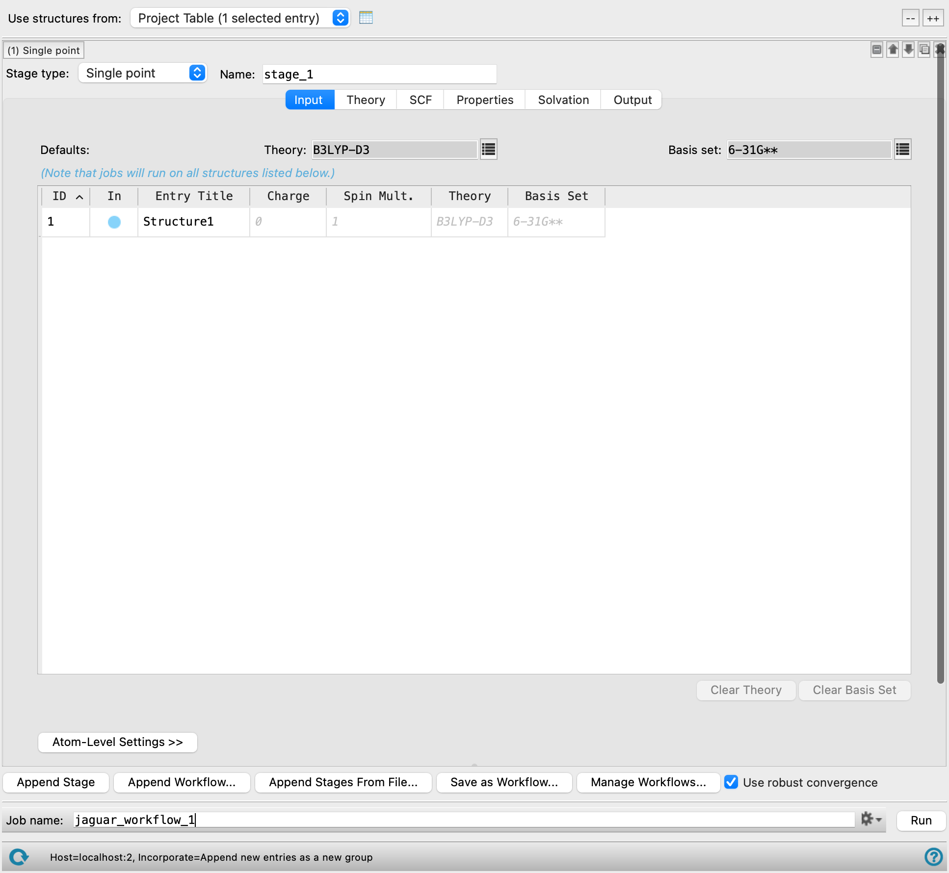
This panel allows you to set up a workflow consisting of multiple sequential QM calculations (run with Jaguar), which is applied to multiple molecules. The settings for each calculation can be set up just as in the Jaguar panel. The Input tab allows you to make molecule-specific settings. The structures listed in this tab are those specified with the Use structures from option menu, and so are the same for each stage. The settings for these structures can be different for each stage, however. In addition, you can add analysis stages for the calculation of properties that are obtained by linear combination of property values from multiple preceding stages.
Workflows can be saved and read in. Reading in previously saved stages does not read in any entry-specific information, only the settings that apply to all structures, including additional keywords and extra sections. Workflows are saved in your Schrödinger user resources directory with a _workflow.txt extension.
Changing a stage from one type to another preserves all the current settings for that stage as long as those settings are relevant for the new stage. For instance, changing Single point to Optimization preserves all settings. Changing from Optimization to Single point and back to Optimization does not preserve Optimization tab settings because they are lost with the switch to the Single point stage.
When the job is run, each stage for each input structure is submitted to the queueing system for execution in the proper sequence. When all the parent stages for a particular stage have finished, the stage is submitted to the queue, subject to any limits on the number of subjobs. You can use multiple processors to distribute subjobs for each entry, and multiple threads to run each calculation with multithreading.
When the job finishes, the structures produced by all stages for all input structures are incorporated into the project. All the project entries are in a parent group named for the job. Within that group, each of the input entries has its own subgroup, and within each subgroup, the entries for the output structures are ordered by stage. However, if there is only one stage, there is only one group, with no subgroups, and naming of output structures does not append a stage identifier.
If subjobs fail for some structures, you can import these structures from the jobname_failed.maegz file. Each structure has a set of Successful step-name Boolean properties, which you can use to determine which steps in the workflow failed. As these are secondary properties you will have to show them in the Project Table first—see Organizing Properties for more information.
To write out the input file and a script for running the job from the command line, click the arrow next to the Settings button  and choose Write.
For properties that involve vibrational frequencies (such as free energies), you might want to make the calculation for specific isotopes. See Changing Atom and Residue Properties for information on setting isotope mass numbers.
QM Multistage Workflow Panel Features
- Structure source
- Collapse/expand all buttons
- Stage management
- Jaguar calculation stage
- Analysis stage
- Stage and workflow buttons
- Reset and Save buttons
- Job toolbar
- Status bar
Structure source
Choose the source of initial structures for the calculations.
- Use structures from option menu
-
Choose the structure source for the current task.
- Project Table (n selected entries)—Use the entries that are currently selected in the Project Table or Entry List. The number of entries selected is shown on the menu item.
- Workspace (n included entries)—Use the entries that are currently included in the Workspace, treated as separate structures. The number of entries in the Workspace is shown on the menu item.
- Project Table (n selected entries)—Use the entries that are currently selected in the Project Table or Entry List. The number of entries selected is shown on the menu item.
- Open Project Table button
-
Open the Project Table panel, so you can

Collapse/expand all buttons
These two buttons (labeled -- and ++) allow you to collapse all workflow stages or expand all workflow stages. When expanded, a scroll bar allows you to navigate the stages.
Stage Management
The main part of the panel has a list of workflow stages, which are executed in the sequence that they appear in this list. The features for management and selection of the stage are described here. The features of each stage are described in the sections below.
- Stage label
-
The label indicates the stage number and the type of the stage. It is updated if the stage type is changed or the stage is moved. If the stage settings are hidden, the label gives a brief summary of the main stage parameters.
- stage management buttons
-
These buttons perform display and ordering operations on the stage. They allow for easy duplication and rearrangement of stages.


Show or hide the contents of the stage. When hidden, only the stage number, label (if any) and these buttons are displayed. This is useful when you have a number of stages and want to compare two separate stages, for example. 
Delete the stage. You can collapse or expand all stages with the buttons at the top right of the panel.
- Stage type option menu
-
Choose the type of calculation to be run for this stage of the workflow. The choices are Single point, Optimization, Transition state, and Analysis. The controls that are displayed for the stage depend on the choice you make from this option menu, and the choice is displayed in the label at the top of the stage. The controls for the first three stage types are described under Jaguar calculation stage, and the controls for the Analysis stage are described under Keywords text box.
- Name text box
-
Specify a name for the current stage. The stage name is appended to any file names and structure titles associated with that stage. If there are two or more stages, the Name text box cannot be blank and different names must be specified for each stage. If there is only one stage and you do not specify a custom name (i.e., the text box is blank or left as the default name "
stage_1"), no stage name is appended to file names and structure titles.
Jaguar calculation stage
These stages run Jaguar single point, optimization, and transition state calculations.
- Geometry from stage option and box
-
Select this option to use the geometry from the stage specified in the box. If this option is not selected, the geometry used is taken from the structure source as specified with the Use structures from option menu. The Wavefunction and Hessian options are only available when this option is selected.
- Wavefunction option
-
Use the wave function from the stage specified with the Geometry from stage option and box.
- Hessian option
-
Use the Hessian from the stage specified with the Geometry from stage option and box.
- Settings tabs
-
These tabs are the same as in the Jaguar panel, except for the Transition State tab. The Transition State tab only has the controls for the search itself: the controls for selecting the type of search and the structures are absent because only a single structure can be given, and the controls for settings made in the Input tab are also absent. This means that the search is a standard search, applied to the input structure.
- Input
- Transition State
- Theory
- SCF
- Optimization
- Properties
- Solvation
- Output
Input Tab Features
- Use structures from option menu
- Open Project Table button
- Defaults tools
- Structures table
- Atom-Level Settings button
- Use structures from option menu
-
Choose the structure source for the current task.
- Project Table (n selected entries)—Use the entries that are currently selected in the Project Table or Entry List. The number of entries selected is shown on the menu item.
- Workspace (n included entries)—Use the entries that are currently included in the Workspace, treated as separate structures. The number of entries in the Workspace is shown on the menu item.
- Project Table (n selected entries)—Use the entries that are currently selected in the Project Table or Entry List. The number of entries selected is shown on the menu item.
- Open Project Table button
-
Open the Project Table panel, so you can
- Defaults tools
-
These tools allow you to specify the default basis set and the default level of theory.
- Theory text box and button
-
Click the button to select the level of theory. A small pane opens with controls for selecting the level of theory. The pane consists of a search text box, a filter button, and a list of available theoretical models. Typing in the text box narrows the list to items that contain the text. Clicking the filter button allows you to set options to restrict the list to certain models, e.g. range-corrected DFT. When you choose an item from the list, the pane closes and the text box (which is noneditable) shows the level of theory you chose.
-
Making a choice of functional sets the dftname keyword in the gen section of the input file.
-
See DFT Keywords in the Jaguar Input File for information on the density functionals.
- Basis set text box and button
-
Click the button to select the basis set. A small pane opens with controls for selecting the basis set. The pane consists of a search text box, a filter button, and a list of basis sets. Typing in the text box narrows the list to basis set names that contain the text. Clicking the filter button allows you to set options to restrict the list to basis sets with certain features: ECP, diffuse functions, pseudospectral, relativistic, RI-MP2 compatible. When you choose a basis set from the list, the pane closes and the text box (which is noneditable) shows the basis set you chose.
See Basis Sets for information on the basis sets available.
- Structures table
-
This table lists the entries in the Project Table that are used as the input structures for the job, according to the choice from the Use structures from option menu. To change the structures used for the calculation, you can change the selected structures or included structures in the Project Table panel or the Entry List panel. You can double-click in a cell to edit the values (ID, In, and Entry Title columns are not editable). The columns of the table may be different depending on the calculation type, and include:
- ID—The entry ID of the structure.
- In—Use this column to display the structures in the Workspace, just as in the Project Table panel or the Entry List panel. If you chose Workspace as the source of structures, excluding structures from the Workspace (clearing the In box) removes them from the table.
- Entry Title—The entry title of the structure.
- Charge—Specify the charge (molchg in the gen section). Default is 0 and is displayed in italics. The value is stored as a Maestro property.
- Spin Mult.—Specify the spin multiplicity (multip in the gen section). Default is 1 (singlet) and is displayed in italics. If you use the spin-orbit ZORA Hamiltonian, spin is no longer conserved, and the multiplicity is only related to the number of electrons (1 for even, 2 for odd). The value is stored as a Maestro property.
- Theory—Specify the level of theory (dftname in the gen section) for each structure. Double-click in a cell to edit the level of theory. A small window is displayed with controls for selecting the functional. These controls are the same as for setting the default theory (see above), except that functionals that are not available for the molecule are dimmed.
- Basis set—Specify the basis set (basis in the gen section) for each structure. Double-click in a cell to edit the basis set. A small window is displayed with controls for selecting the basis set. These controls are the same as for setting the default basis set (see above), except that basis sets that are not available for the molecule are dimmed. The tooltip for the cell shows the basis set and the number of basis functions for the structure. If a composite method is chosen in the Theory column, the corresponding pre-defined basis set is used and the cell becomes noneditable.
- Atom-Level Settings button
-
Click this button to show or hide the controls for making settings at the atomic level for the selected molecule in the selected entries table.
- Per-Atom Basis tab
-
In this tab, you can set the basis set for individual atoms. The tab has a Pick atoms option, which you select to pick the atoms in the Workspace that you want to assign a basis set to. Each pick adds an atom to the table, which shows the atom label, the entry ID, the entry title, and the basis set. You can select the basis set in the same way as in the selected entries table, by double-clicking in the table cell, and choosing the basis set in the window that appears. The basis sets are added to the atomic section of the input file.
- Charge Constraints tab
-
In this tab, you can specify one or more groups of atoms whose net charge is constrained to a particular value. The constraint is applied using the constrained DFT method, and the atoms are defined by Becke's partitioning of atomic volumes [277]. This feature is useful for localizing the charge on part of a molecule, or one molecule in a dimer, for example. To set up a constraint, click New Constraint, pick the atoms for the constraint in the Workspace, then edit the Charge cell to set the net charge on the atoms. A small table appears below the cell so you can set weights for the individual atoms in the constraint. This table is displayed in the tooltip for the cell so you can view the weights. The constraints are added to the cdft section of the input file.
Transition State Tab Features
In this tab you select the transition state search method and the structures that define reactant and product, and set parameters for the search. You also make settings for the symmetry and molecular state, and choose a basis set.
- Search controls
-
Specify the direction to search in standard and LST searches.
- Search along option menu
-
Choose the direction to search from the initial structure. Sets itrvec in the gen section.
Under certain circumstances, you might want to direct your transition-state search using these options, rather than having the optimizer simply minimize along the lowest Hessian eigenvector found for each iteration. The Lowest non-torsional mode and Lowest bond-stretch mode options can be useful for steering the optimizer to a particular type of transition state—for instance, for a study of a bond-breaking reaction, you can avoid converging to a torsional transition state by choosing Lowest bond-stretch mode.
The options are:
- Lowest Hessian eigenvector
-
Follow the lowest Hessian eigenvector, excluding the trivial (rotational and translational) modes. Not available for QST searches. Sets itrvec=0.
- Lowest non-torsional mode
-
Follow the lowest non-torsional mode derived from the initial Hessian. Not available for QST searches. Sets itrvec=-1.
- Lowest bond-stretch mode
-
Follow the lowest mode derived from the initial Hessian that corresponds to a bond stretch. Not available for QST searches. Sets itrvec=-2.
- Reactant-product path
-
Follow the path between the supplied reactant and product structures. Not available for standard searches. Sets itrvec=-5.
- User-selected eigenvalue
-
Follow the mode defined by an eigenvalue of the initial Hessian, by specifying the index of the eigenvalue in the Eigenvector text box. Not available for QST searches. Sets itrvec to the value in the text box.
- Active coordinate eigenvalue
-
Follow the eigenvalue that contains the largest weight of the active coordinates specified in the Optimization tab. Not available for QST searches. Sets itrvec=-6.
- Eigenvector text box
-
Specify the eigenvector of the initial Hessian to follow in the search. Only available if you select User-selected eigenvalue from the Search along option menu.
You can identify the index number by running one geometry optimization iteration (see SCF and Geometry Convergence for more information) and examining the output summary of the Hessian eigenvectors, which indicates the dominant internal coordinates and their coefficients for each eigenvector.
- Follow same eigenvector option
-
Follow the eigenvector of the Hessian that has the largest overlap with the eigenvector followed in the previous step. This option is useful because the order and the character of the eigenvectors can change during an optimization. Sets ifollow=1 in the gen section. This option is set and cannot be changed if you select User-selected eigenvalue from the Search along option menu.
If this option is not set, the optimization follows the eigenvector of the same index number as the previous iteration.
- Hessian refinement option and controls
-
Select this option to turn on Hessian refinement, then choose an option for the target of the refinement. Refinements involve SCF and gradient calculations for displacements along these modes, which allow more accurate information about the most important modes to be included in the Hessian.
- Low-frequency modes—refine the modes of the lowest frequency. Enter the number of eigenvectors of the Hessian to use in the refinement in the text box. The eigenvectors are counted from the lowest nontrivial mode. Sets nhesref=3 in the gen section
- Use active coordinates—refine the Hessian for the active coordinates specified in the Optimization tab. This option is only available if active coordinates are specified. Sets nhesref=-1 in the gen section.
With the standard search method, if a coordinate with a negative force constant (Hessian eigenvalue) exists, it is critical for this transition vector to be properly identified as efficiently as possible, since it leads to the transition state. When the initial Hessian chosen is a guess Hessian (one not calculated numerically or read from a restart file), it can be helpful to refine the Hessian during the calculation before using it to compute any new geometries.
Hessian refinement is especially likely to improve transition-state optimizations that employ eigenvector following, because any eigenvector selected for following should be accurate enough to be a reasonable representation of the final transition vector.
See Specifying Coordinates for Hessian Refinement for information on making Hessian refinement settings in the input file.
Theory Tab Features
In this tab, you select options for the level of theory used in the calculation—SCF, DFT, LMP2. The controls displayed in this tab depend on the level of theory selected.
- Theory settings for option menu
- SCF Spin treatment options
- Excited state controls
- Grid density option menu
- Use 3-body dispersion correction with all applicable dispersion-corrected functionals option
- Core localization method option menu
- Valence localization method option menu
- Resonance option menu
- LMP2 Pairs options
- Hamiltonian option menu
- Theory settings for option menu
-
Select an option from this menu to make settings for the three types of theoretical methods used: Hartree-Fock (HF), density functional theory (DFT), and local second-order Møller-Plesset perturbation theory (LMP2). The controls in the rest of the tab depend on the choice you make from this menu.
-
SCF and DFT options
-
Set options for SCF and DFT calculations.
- SCF Spin treatment options
-
The treatment of spin restriction in the SCF process can be controlled by three options.
-
Automatic—run a spin-unrestricted calculation for open-shell systems (multip>1) and a spin-restricted calculation for closed-shell systems (multip=1). Sets iuhf=2 in the gen section.
-
Unrestricted—run a spin-unrestricted (UHF or UDFT) calculation for both closed-shell and open-shell systems. For closed-shell systems this may give the same result as a restricted calculation, but can deviate from it where a single determinant is no longer a good description of the wave function. Sets iuhf=1 in the gen section.
-
Restricted—run a spin-restricted (ROHF or RODFT) calculation for open-shell systems (sets iuhf=0 in the gen section).
These options are only displayed if you choose HF (Hartree-Fock) or DFT (Density functional theory) from the Level of theory option menu. The default is Automatic: unrestricted for open-shell HF or DFT calculations, restricted for closed-shell calculations.
When using the spin-orbit ZORA Hamiltonian, the spin is no longer conserved. Time-reversal symmetry takes the place of spin symmetry, and Kramers restriction takes the place of spin restriction. So choosing Restricted runs a Kramers-restricted SCF calculation (where time-reversal symmetry is imposed), and Unrestricted runs a Kramers-unrestricted SCF calculation.
-
- Excited state controls
-
Select the Excited state option to perform an excited state calculation using either the time-dependent density-functional method (TDDFT), if the level of theory is DFT, or the time-dependent Hartree-Fock (TDHF) method, if the level of theory is HF. (Note that the option label includes (TDHF) or (TDDFT) to distinguish the two levels of theory.) This option sets itddft=1 in the gen section. For a geometry optimization, this option is labeled Optimize first excited state to indicate that only the lowest excited state is optimized.
The full linear response method is used by default. If you want to use the Tamm-Dancoff approximation, you can choose it from the option menu (itda=1 in the gen section). For TDHF, this corresponds to a configuration interaction singles (CIS) calculation.
The excited states are excitations from a reference state. If the reference state is a closed shell, you can choose whether to generate singlet or triplet excited states, or both, from the Excited state type option menu. (These choices set rsinglet=1 and rtriplet=1 in the gen section). This option menu is not available if you are doing a geometry optimization. If the reference state is a spin-unrestricted open-shell state, all possible spin states that are accessible as single excitations are calculated, but there is no classification of these states by spin. The value of S2 is reported for all states, so you can identify the spin state.
You can calculate excited states with both the scalar ZORA and the spin-orbit ZORA Hamiltonians (see the Hamiltonian option menu). For the scalar ZORA Hamiltonian, all the options are available. The spin-orbit ZORA Hamiltonian generates states of mixed spin, so the Excited state type option menu is not available when you choose this Hamiltonian. You can only use the spin-orbit ZORA Hamiltonian with a closed-shell reference state. This Hamiltonian is useful if you are interested in singlet-to-triplet transitions and phosphorescence lifetimes.
Several settings can be made for the excited state methods, which are only available when you select the Excited state option.
- Number of excited states text box
-
Specify the number of excited states (sets nroot). Note that for a geometry optimization, only the lowest singlet excited state is optimized, regardless of the value in this text box.
You should select more excited states than you are actually interested in, for two reasons. The first is that the initial guess might not accurately reflect the final states, and the second is to ensure that near-degeneracies are accounted for.
- Maximum TDHF iterations text box
- Maximum TDDFT iterations text box
-
Specify the maximum number of iterations of the diagonalization procedure (sets mitertd).
- Energy convergence threshold text box
-
Specify the threshold used to determine when the energies of the excited states have converged (sets econtd).
- Residual convergence threshold text box
-
Specify the threshold used to determine when the norm of the residual vector for the excited states has converged (sets rcontd).
The excited state controls are only displayed if you choose HF (Hartree-Fock) or DFT (Density Functional Theory) from the Level of theory option menu.
- Grid density option menu
-
Choose the grid density for the DFT calculation, from Medium, Fine, or Maximum. If you read an input file that contained some other grid density, the grid density is set to Other, otherwise this option is unavailable. If you choose a grid density from this menu, the previous grid density specification is replaced. By default, DFT calculations use grids with a medium point density.
This option menu is only displayed if for DFT methods.
- Use 3-body dispersion correction with all applicable dispersion-corrected functionals option
-
Select this option to include an additional correction for three-body effects for any D3 dispersion-corrected functionals. Only present if you choose DFT (Density Functional Theory) from the Level of theory option menu.
-
LMP2 Options
-
Set options for LMP2 calculations. See Local MP2 Settings for more information on the method and its settings.
- Core localization method option menu
-
Choose the localization method for the core orbitals from this option menu.Sets loclmp2c in the gen section. This menu is only displayed if you choose LMP2 (Local MP2) from the Level of theory option menu. The options are:
- None—Do not localize core orbitals (loclmp2c=0). This is the default.
- Pipek-Mezey—Perform Pipek-Mezey localization, maximizing Mulliken atomic populations (loclmp2c=2).
- Boys—Perform Boys localization (loclmp2c=1).
- Pipek-Mezey (alt)—Perform Pipek-Mezey localization, maximizing Mulliken basis function populations (loclmp2c=3).
- Valence localization method option menu
-
Choose the localization method for the valence orbitals from this option menu. Sets loclmp2v in the gen section. This menu is only displayed if you choose LMP2 (Local MP2) from the Level of theory option menu. The options are
- Pipek-Mezey—Perform Pipek-Mezey localization, maximizing Mulliken atomic populations (loclmp2v=2). This is the default.
- Boys—Perform Boys localization (loclmp2v=1).
- Pipek-Mezey (alt)—Perform Pipek-Mezey localization, maximizing Mulliken basis function populations (loclmp2v=3).
- Resonance option menu
-
Choose the handling of resonance structures for aromatic molecules and molecules with conjugated double bonds. Sets ireson in the gen section. This menu is only displayed if you choose LMP2 (Local MP2) or from the Level of theory option menu. The options are:
- None—Do not delocalize LMP2 pairs over other atoms (ireson=0).
- Partial delocalization—Delocalize LMP2 pairs over neighboring atoms in aromatic rings (ireson=1).
- Full delocalization—Delocalize LMP2 pairs over all atoms in aromatic rings (ireson=2).
- LMP2 Pairs options
-
Select the types of LMP2 pairs to include in the calculation. Sets iheter in the gen section. This menu is only displayed if you choose LMP2 (Local MP2) from the Level of theory option menu. The options are:
- All atom pairs—Treat all atom pairs with LMP2 (iheter=0). This is the default.
- Hetero atom pairs—Treat atom pairs in which the two atoms are different (except CH pairs) with LMP2 (iheter=1).
-
RI-MP2 Options
-
Set options for RI-MP2 calculations. See RI-MP2 Calculations for more information on the method and its settings.
- Freeze core option
-
Select this option to freeze core molecular orbitals (n_frozen_core = -1). The number of orbitals Jaguar freezes by default for each atom is listed here. If this option is not checked, all core molecular orbitals are included in the correlation.
- Hamiltonian option menu
-
For heavy elements, it is necessary to include relativistic effects in the Hamiltonian. In Jaguar there are two ways of doing this: using ECPs, and with an explicit relativistic Hamiltonian. ECPs are handled via the basis set selection. The Hamiltonian option menu allows you to choose the Hamiltonian. The default is Nonrelativistic, which is the usual Schrödinger Hamiltonian. The other choices are for relativistic Hamiltonians, and include (relativistic) in the menu item, to indicate that they include relativistic effects.
-
Nonrelativistic—Use the (nonrelativistic) Schrödinger Hamiltonian. This is the default, and should be used with ECPs. If you choose LMP2 for the level of theory, this Hamiltonian is selected, as LMP2 cannot currently be used with ZORA.
-
Scalar ZORA—Use the scalar ZORA Hamiltonian (relham=zora-scalar or zora-1c in the gen section). This option is only available for single-point HF and DFT calculations. If you choose this option for LMP2, the Level of theory is reset to DFT.
-
Spin-orbit ZORA—Use the spin-orbit ZORA Hamiltonian (relham=zora-so or zora-2c in the gen section). The Hamiltonian includes spin-orbit coupling, which mixes states of different spin and spatial symmetry. Properties are not available with this Hamiltonian. This option is only available for single-point HF and DFT calculations. If you choose this option for LMP2, the Level of theory is reset to DFT.
Both of the ZORA Hamiltonians use a one-center approximation for the ZORA integrals, with the potential taken from the atomic initial guess (potential=local in the relativity section). By default the ZORA integrals are only evaluated for elements with Z > 18; lighter atoms are treated nonrelativistically. You can override this by including a relatom keyword in the relativity section, set to a space- or comma-separated list of elements, e.g.
relatom=C N O F.For ZORA calculations, it is recommended that you choose a heavy-atom basis set that is contracted specifically for ZORA. These basis sets have zora in the name. The dyall-v2z_zora-j-pt-gen basis set is a double-zeta polarized basis set similar to cc-pvdz; the dyall-2zcvp_zora-j-pt-gen basis set adds outer core polarization. Both basis sets are generally contracted, and cover elements up to Rn. There are semi-segmented versions of these basis sets that run faster without loss of accuracy, dyall-v2z_zora-j-pt-seg and dyall-2zcvp_zora-j-pt-seg. The sarc-zora basis set is also of double-zeta quality, and is a segmented contraction, covering elements from La to Rn. For a higher quality, you can use the dyall-3zvp_zora-j-pt-seg and dyall-3zcvp_zora-j-pt-seg basis sets, which are triple-zeta basis sets.
-
SCF Tab Features
In this tab you set the parameters that control the SCF convergence. Keywords for the gen section of the input file that correspond to the controls in this tab are given in parentheses.
- Accuracy level option menu
- Initial guess option menu
- Convergence criteria section
- Convergence methods section
- Orbitals section
- Accuracy level option menu
-
Set the accuracy for pseudospectral calculations, or turn off the pseudospectral method.
- Quick— Use mixed pseudospectral grids with loose cutoffs (Sets iacc=3).
- Accurate— Use mixed pseudospectral grids with accurate cutoffs (Sets iacc=2).
- Ultrafine— Use ultrafine pseudospectral grids with tight cutoffs (Sets iacc=1).
- Fully analytic— Perform a fully analytic calculation: turn off the pseudospectral method (Sets nops=1). Can be run in parallel with OpenMP threads—see Running a Multithreaded Jaguar Job with OpenMP.
-
For more information on grids and cutoffs, see The Grid File for Jaguar Calculations and The Cutoff File for Jaguar Calculations.
- Initial guess option menu
-
Choose the method for generating an initial guess for the molecular orbitals.
-
Atomic overlap—Construct a guess for the molecular orbitals from atomic orbitals (iguess=10). The core orbitals are set to the atomic core orbitals. The overlap matrix is diagonalized in the space of the valence atomic orbitals, and the eigenvectors with the largest eigenvalues are taken for the valence orbitals. The entire set is orthogonalized core first, then valence. This is the default.
-
Atomic density—Construct a guess from a superposition of atomic densities (iguess=11). The density is projected onto the AO basis. The resulting matrix is diagonalized to give natural orbitals, which are used as the initial guess orbitals.
-
Core Hamiltonian—Generate an initial guess by diagonalizing the one-electron Hamiltonian matrix (iguess=0). This is rarely a good guess, as the orbitals are usually too tight.
-
Ligand field theory—For transition metal complexes, use ligand field theory to construct an initial guess for the metal d orbitals. (iguess=25) An effective Hamiltonian is diagonalized, taking into account the assigned formal charges on the metal and the ligand and the occupation of the ligand orbitals, to determine the d-orbitals and the orbital ordering. The core and ligand orbitals are determined from the atomic orbitals using the atomic overlap.
-
Ligand field theory with d-d repulsion—For transition metal complexes, use ligand field theory including d-d repulsion to construct an initial guess (iguess=30). The procedure is the same as above, except that repulsion between the d electrons on the metals is included to determine the orbital ordering and hence the occupation of the d orbitals and the spin state.
-
- Convergence criteria section
-
In this section you set the criteria for convergence of the SCF process.
- Maximum iterations text box
-
Specify the maximum number of SCF iterations in this text box (maxit). The default value is 48. The absolute maximum allowed is 5000.
- Energy convergence text box
-
Specify the SCF energy convergence threshold in this text box (econv). The default value is 5.0x10⁻⁵ Eh.
- RMS density matrix change text box
-
Specify the SCF density convergence threshold in this text box. This value is the maximum change in the RMS density difference between iterations. (dconv). The default value is 5.0x10⁻⁶.
- Convergence methods section
-
In this section you choose the methods used to enhance or control convergence.
- SCF level shift text box
-
Specify the level shift for the virtual orbitals (vshift). The default value is 0.0 for non-metallic systems and Hartree-Fock calculations. For DFT calculations on metallic systems the default is 0.2 for hybrid functionals, 0.3 for pure functionals.
- Thermal smearing option menu
-
Select the thermal smearing method for convergence control (ifdtherm). The menu options are:
- None— Do not use thermal smearing (ifdtherm=0).
- FON— Fractional occupation number method (ifdtherm=1).
- pFON— Pseudo-fractional occupation number method (ifdtherm=2).
See the Jaguar User Manual for details of this method.
- Initial temperature text box
-
Set the initial temperature for thermal smearing. (fdtemp in the gen section of the input file). The initial temperature text box is only available if you choose an item other than None from the Thermal smearing option menu.
- Convergence scheme option menu
-
Choose the SCF convergence acceleration scheme (iconv).
- DIIS— Use the DIIS convergence scheme (iconv=1).
- OCBSE— Use the OCBSE convergence scheme (iconv=3).
- GVB-DIIS— Use the GVB-DIIS convergence scheme (iconv=4).
- Other— Selected if the input file uses another convergence scheme, otherwise unavailable.
For more information on these convergence schemes, see the Jaguar User Manual.
- Force convergence option
-
Attempt to force convergence by adding level shift and decreasing it during iterations, fixing the number of canonical orbitals, and running at ultrafine accuracy (vshift, iacscf=1).
- Compute wave function stability option
-
Perform wave function stability analysis (wf_stability = 1). Eigenvalues of the diagonalized molecular orbital Hessian are reported.
- Orbitals section
-
Set options relating to the orbital occupations, canonicalization, and localization.
- Fixed symmetry populations option
-
Fix the number of electrons in each irreducible representation (ipopsym=1).
- Use consistent orbital sets when all input structures are isomers option
-
When performing calculations on a set of isomers, taken either from the project table or from a file, select this option to ensure that all calculations use the same number of canonical orbitals. This ensures consistency of the calculations and enables the results to be validly compared.
This option is not present in the Jaguar - Reaction panel, as the structures are not isomeric.
- Final localization option menu
-
Choose the localization method for the valence orbitals from this option menu (locpostv).
- None— Do not localize final valence orbitals (locpostv=0). This is the default.
- Pipek-Mezey— Perform Pipek-Mezey localization, maximizing Mulliken atomic populations (loclpostv=2).
- Boys— Perform Boys localization (loclmp2c=1).
- Pipek-Mezey (alt) Perform Pipek-Mezey localization, maximizing Mulliken basis function populations (locpostv=3).
Optimization Tab Features
In this tab you set parameters that control the optimization of geometries, and set constraints on geometric parameters in the optimization.
- Maximum steps text box
- Switch to analytic integrals near convergence option
- Convergence criteria option menu
- Initial Hessian option menu
- Coordinates option menu
- Save intermediate geometries to output structure file option
- Add New Constraint section
- Constraints table
- Maximum steps text box
-
Enter the maximum number of geometry steps to be taken in the optimization. (Sets maxitg.)
Many molecules will meet the convergence criteria after ten or fewer geometry iterations. Input containing very floppy molecules, transition metal complexes, poor initial geometries, or poor initial Hessians may require many cycles to converge.
- Switch to analytic integrals near convergence option
-
When the optimization approaches convergence, switch to using analytic integrals rather than the pseudospectral method. This option is useful for cases where tight convergence is required, as the pseudospectral method may not provide sufficient accuracy. The switch is made when the quantities used to assess convergence are within a factor of 10 of the relevant convergence threshold (sets nops_opt_switch=10
- Convergence criteria option menu
-
Set the convergence criteria for geometry optimizations. See Geometry Optimization and Transition-State Keywords in the Jaguar Input File for details of the criteria.
- Loose—These thresholds are five times larger than the default thresholds. (Sets iaccg=3.)
- Normal— Set the convergence criteria to the defaults. (iaccg is not set and different defaults are used depending on the system.)
- Accurate—Set the convergence criteria to the defaults, given in Table 7 in Geometry Optimization and Transition-State Keywords in the Jaguar Input File. (Sets iaccg=2.)
- Tight—These thresholds are ten times smaller than the default thresholds. (Sets iaccg=5.)
- Custom—The Energy change, Gradient RMS, and Maximal displacement RMS text boxes are displayed, so you can enter the values you want to use for these criteria.
For optimizations in solution, the default criteria are multiplied by a factor of three, and a higher priority is given to the energy convergence criterion.
- Initial Hessian option menu
-
Choose an initial guess for the Hessian. Sets inhess in the gen section. The choices are:
-
Fischer-Almlof—Use the Fischer-Almlof initial guess. Sets inhess=-1.
-
Schlegel—Use the Schlegel initial guess (the default). Sets inhess=0.
-
Unit Hessian—Use the unit matrix for the initial Hessian. Sets inhess=1.
-
Quantum mechanical—Calculate the Hessian with the given basis set. This is the most expensive but most accurate option, recommended for floppy molecules and other molecules that are difficult to optimize. Sets inhess=4.
-
Other—Read the Hessian from the input file hess section if it exists (see The hess Section of the Jaguar Input File). Otherwise use the default. Automatically selected if the input file has a Hessian, which is the case for restarting a geometry optimization. Sets inhess=2.
-
- Coordinates option menu
-
Choose a coordinate representation to define the optimization parameters. Sets intopt in the gen section. The ideal set of coordinates is one in which the energy change along each coordinate is maximized, and the coupling between coordinates is minimized. The choices are:
-
Redundant internal—Use internally-generated redundant internal coordinates for the optimization parameters. Sets intopt=1. This is the default, and the most efficient choice in most cases. New coordinates are chosen automatically if a group of atoms becomes collinear.
-
Cartesian—Use Cartesian coordinates for the optimization parameters. Sets intopt=0. Avoids the problems of collinear coordinate sets, but is likely to take longer than for redundant internal coordinates.
-
Z-matrix—Use the Z-matrix from the input file for the optimization parameters. Sets intopt=2. If the geometry input is in Cartesian format or contains a second bond angle rather than a torsional angle for any atom intopt is set to 1. This item is unavailable if you are doing an IRC calculation.
-
- Save intermediate geometries to output structure file option
-
Save the geometry at each step of the optimization to the output structure file. The structures at each geometry step are imported into Maestro as an entry group. If the geometry optimization fails, you can select one of these structures in Maestro to restart the optimization. Sets ip472=2 in the gen section. You do not need to set this option to inspect the energy convergence, which you can do in the QM Monitor Panel.
- Add New Constraint section
-
Choose a constraint type and pick atoms in the Workspace to define the constraint. When you have picked the required number of atoms for the constraint type, the constraint is listed in the Constraints table. Cartesian constraints are marked with an asterisk in the zmat section; distance, angle, and dihedral constraints are added to the coord section, which is created if it does not exist. You can also choose to add all constraints of a particular type.
- Type option menu
-
Choose the type of constraint. Choices are Cartesian X, Cartesian Y, Cartesian Z, Cartesian XYZ, Distance, Angle, and Dihedral. The Cartesian constraints constrain movement in the specified direction (X, Y, Z, or all three).
- Pick option and menu
-
Choose an object from this option menu, then pick atoms in the Workspace to define the constraint. When you choose from this menu, the Pick option is automatically selected. The available objects are Atoms for Cartesian constraints, and Atoms and Bonds for all other types of constraint. The atoms are marked in the Workspace as you pick them, and each constraint is marked in the Workspace and entered in the Constraints table as it is completed.
- Add object button
-
This button adds all of the specified object type to the constraints table. It is mainly useful when you want to optimize only a small part of a molecule, which you can do by constraining the whole system, then deleting those constraints that you don't want. The button's label and function depend on the choice you make from the Type option menu:
-
Add Selected Atoms—Add the atoms that are selected in the Workspace as constraints. Only available for Cartesian constraints. You can select atoms in the Workspace then click this button to add them to the constraints table.
-
Add All Atom Pairs—Add all atom pairs in the molecule as constraints, whether bonded or not. This choice completely constrains all free parameters, so it is only useful as a first step to removing constraints on the atoms you want to move. Only available for distance constraints.
-
Add All Bond Angles—Add all bond angles in the molecule, i.e. all angles in which the atom at the apex of the angle is bonded to the two other atoms. Only available for angle constraints.
-
Add All Torsions—Add all bonded torsions in the molecule, i.e. all dihedrals defined by three contiguous bonds. Only available for dihedral constraints.
-
- Constraints table
-
Displays the constraints with their type, and also the target value, if it is a dynamic constraint. You can select one row at at time in the table. The constraint for the selected row is highlighted in the Workspace. You can make a constraint dynamic by entering the desired value in the Target Value column.
You can delete a constraint by selecting it in the table and clicking Delete. To remove all constraints, click Delete All.
Properties Tab Features
In this tab, you select the properties you want to calculate and set any relevant options.
The tab consists of a table listing all the available properties, and controls for each of the properties that are displayed in the lower portion of the tab when you select the row for the property in the table.
- Properties table
- Vibrational frequencies controls
- Surfaces controls
- Electrostatic potential option
- Average local ionization energy option
- Energy units option menu
- Noncovalent interactions option
- Noncovalent grid density text box
- Electron densities options
- Spin density option
- Molecular orbitals option
- NTO for excited states option
- Box size adjustment text box
- Grid density text box
- Atomic electrostatic potential charges controls
- Mulliken populations controls
- NBO analysis controls
- Multipole moments controls
- Polarizability/Hyperpolarizability controls
- NMR shielding constants controls
- Atomic Fukui indices controls
- Stockholder charges controls
- Vibrational circular dichroism controls
- Electronic circular dichroism controls
- Raman spectroscopy controls
- Mössbauer controls
Properties Table
The properties table lists all the properties that can be selected for calculation. Properties that are not available with the chosen level of theory are grayed out in the table.
To set options for a property, click the row containing the property. The controls for the property are displayed in the lower portion of the panel. If the property is not available for the chosen level of theory, the controls are displayed but are not available.
To select a property for calculation, click the check box in the Calculate column for the property.
Vibrational Frequencies Controls
Set options for vibrational frequency and thermochemistry calculations. See Jaguar Vibrational Frequencies for details.
- Use available Hessian option
-
Select this option if there is a Hessian available in the input file and you want to use it to calculate the frequencies. Sets ifreq = −1 in the gen section. Otherwise, the Hessian is calculated. The Hessian from a geometry optimization is not usually accurate enough for frequency calculations.
- IR intensities option
-
Calculate infrared and Raman intensities. Only available for closed-shell wave functions. Sets irder = 1 in the gen section. See Infrared and Raman Intensities for more information.
- Atomic masses option menu
-
Select the option for the atomic masses used in the frequency calculations. Sets massav in the gen section. The choices are:
- Most abundant isotopes
- Use the mass of the most abundant isotopes (massav = 0). This is the default.
- Average isotopic masses
- Use the average atomic mass (massav = 1).
For information on setting isotopic mass numbers for individual elements, see Changing Atom and Residue Properties.
- Scaling controls
-
Select options for the scaling of the frequencies. The keywords set in the gen section are given for each option. See Scaling of Jaguar Frequencies for more information.
- None
- Do not scale frequencies. This is the default. (isqm = 0)
- Pulay SQM
- Scale frequencies with the Pulay SQM method and use scaled frequencies in thermochemistry calculations (isqm = 1). Only available for B3LYP/6-31G calculations (with or without polarization).
- Automatic
- Scale frequencies using predetermined factors for the basis set and method chosen (auto_scale = 1). Optimized factors are available for a wide range of basis sets and methods.
- Custom
- Scale frequencies using the factor given in the text box, which is displayed when you choose this item (scalfr).
- Thermochemistry controls
-
Set options and values for thermochemical properties (enthalpy, Gibbs energy, entropy, heat capacity, and so on). You can calculate thermochemical properties at a range of temperatures for the given pressure. Along with the total internal energy, total entropy, and total free energy (in hartrees) at the given (or initial) temperature, the thermochemical property values as a function of temperature and pressure are added to the output Maestro file as Maestro properties. They can be plotted in the Thermochemistry Viewer Panel.
- Pressure
- Enter the pressure in atmospheres. The default is 1.0 atm. Sets press in the gen section.
- Start temperature
- Enter the initial temperature in K. The default is 298.15 K. Sets tmpini in the gen section.
- Increment
- Enter the temperature step in K. Sets tmpstp in the gen section.
- Number of steps
- Enter the number of temperature steps. Sets ntemp in the gen section.
- Output units
- Select an option for output in kcal/mol or kJ/mol. The default is kcal/mol (for H and G) and cal/mol K (for Cv and S). Sets eunit in the gen section.
Surfaces Controls
Set options for generating plot data on a 3D grid (a "volume") that is used in Maestro to display surfaces. Plot data is written to a .vis file.
- Electrostatic potential option
-
Calculate the electrostatic potential (ESP) on the grid (sets iplotesp=1 in the gen section). Also performs an analysis of the ESP on an isodensity surface and reports the results in the output file and as entry and atom properties in the Maestro file.
- Average local ionization energy option
-
Calculate the average local ionization energy (ALIE) on the grid (sets iplotalie=1 in the gen section). Also performs an analysis of the ALIE on an isodensity surface and reports the results in the output file and as entry and atom properties in the Maestro file.
- Energy units option menu
-
Select the units used to represent the ESP and the ALIE (sets espunit in the gen section).
- Noncovalent interactions option
-
Calculate reduced density gradient and interaction strength for visualization of noncovalent interactions (sets iplotnoncov=1 in the gen section). See the topic Noncovalent Interactions Overview for an explanation.
- Noncovalent grid density text box
-
Set the grid density for the reduced density gradient and interaction strength points for noncovalent interactions (sets plotresnoncov in the gen section). The default is 20 points per angstrom. A high grid density is needed for good visualization.
- Electron densities options
-
Calculate the electron density and optionally the electron density difference on a grid. The two options are:
-
Density only—Calculate only the electron density for the final converged wave function (sets iplotden=1 in the gen section).
-
Density and density difference—Calculate the final converged electron density function and the electron density difference between the final converged density and the initial guess density (sets iplotden=2 in the gen section). The interpretation of this density difference depends on the initial guess. For example, if the initial guess density is the superposition of atomic densities, then the difference density is the density change on molecule formation. If it is derived from another geometry, it represents the relaxation of the density due to the geometry change.
-
- Spin density option
-
Calculate the electron spin density on the grid (sets iplotden=1 in the gen section). Only available for UHF and UDFT wave functions.
- Molecular orbitals option
-
Calculate the specified molecular orbitals on the grid. Not available for MP2 calculations. Localized orbitals are calculated if the localization was performed.
Choose the references for the molecular orbital indices from the option menus and enter the relative index in the text box.
HOMO -: Count down from the HOMO, inclusive.
LUMO +: Count up from the LUMO, inclusive.
Thus, From: HOMO - 0 To: LUMO + 0 includes both the HOMO and the LUMO. These controls set iorb1a and iorb2a in the gen section. The controls for beta orbitals are only available for UHF and UDFT wave functions, and set iorb1b and iorb2b in the gen section. - NTO for excited states option
-
Calculate natural transition orbitals (NTOs) for each excited state in a TDDFT calculation, and write out the surfaces for each particle and hole NTO with an eigenvalue (occupation) greater than 0.1. Sets tddft_nto to 1 in the gen section.
- Box size adjustment text box
-
Enter a value to adjust the size of the box used to calculate the grid. The default box size encompasses the van der Waals radii of all atoms in the molecule. Sets xadj, yadj and zadj in the gen section.
- Grid density text box
-
Enter the number of grid points per angstrom. Sets plotres in the gen section.
Atomic Electrostatic Potential Charges Controls
Set options for charge fitting to the electrostatic potential. The atomic charges are written to the output Maestro (
.mae) file and are available in Maestro as the partial charge. By default, the values at the nuclei are also added as atom properties to the output Maestro file.For electrostatic potential fitting of an LMP2 wave function, you should also compute a dipole moment for more accurate results, since the charge fitting will then include a coupled perturbed Hartree-Fock (CPHF) term as well. You might also want to constrain the charge fitting to reproduce the dipole moment, as described below. Because the CPHF term is computationally expensive, it is not included in LMP2 charge fitting by default.
- Fit ESP to option menu
-
Choose option for fitting electrostatic potential. Sets icfit in the gen section.
- Atomic centers
- Fit to atomic centers only (icfit=1).
- Atom + bond midpoints
- Fit to atomic centers and bond midpoints (icfit=2).
- Constraints option menu
-
Choose the level of charge and multipole moment constraints applied to the fit. Sets incdip in the gen section. The option All of the above applies each level sequentially (incdip=-1) .For LMP2 wave functions, only dipole moments are available.
Note that the more constraints you apply to electrostatic potential fitting, the less accurately the charge fitting will describe the Coulomb field around the molecule. The dipole moment from fitting only the charges is generally very close to the quantum mechanical dipole moment as calculated from the wave function. Constraining the charge fitting to reproduce the dipole moment is generally not a problem, but you might obtain poor results if you constrain the fitting to reproduce higher multipole moments. However, this option is useful for cases such as molecules with no net charge or dipole moment.
If multipole moment calculations are performed, the moments are also computed from the fitted charges for purposes of comparison.
- Grid type options
-
Select the grid type for calculating the electrostatic potential. For either grid type, points within the molecular van der Waals surface are discarded. The van der Waals surface used for this purpose is constructed using DREIDING [108] van der Waals radii for hydrogen and for carbon through argon, and universal force field [105] van der Waals radii for all other elements. These radii are listed in Table 2 in Keywords in the Jaguar Input File That Specify Physical Properties. The radius settings can be altered by making vdw settings in the atomic section of an input file, as described in The atomic Section of the Jaguar Input File.
- Spherical—Use a spherical grid on each atom, like those used for pseudospectral or DFT calculations. Sets gcharge = −1 in the gen section.
- Rectangular—Use a rectangular grid [107]. Sets gcharge = −2 in the gen section. The grid spacing in bohr is specified in the text box (sets wispc in the gen section).
Mulliken Population Analysis Controls
This section provides three method options for the Mulliken population analysis. Sets mulken in the gen section. See Mulliken Population Analysis for more information.
- By atom—Calculate Mulliken populations by atom (mulken=1).
- By atom and basis function—Calculate Mulliken populations by atom and by basis function (mulken=2).
- Bond populations—Calculate Mulliken bond populations (mulken=3).
NBO Analysis Controls
There are no specific controls for NBO analysis [110, 111]. The default NBO analysis is performed. Adds an empty nbo section to the input file. See Natural Bond Orbital (NBO) Analysis for more information.
Multipole Moments Controls
There are no specific controls for multipole moments. Dipole, quadrupole, octupole and hexadecupole moments are calculated. Sets ldips=5 in the gen section. See Multipole Moments from Jaguar Calculations for more information.
Polarizability/Hyperpolarizability Controls
These controls allow you to specify which polarizabilities are calculated (static or dynamic; alpha, beta, gamma) and which method is used. The polarizabilities are reported in atomic units.
- Static option
-
Calculate the specified static polarizabilities with the chosen method. The trace of the polarizability tensor (alpha) is reported as an entry property, Polarizability.
- Property / Method option menu
-
Select the combination of property and method. Alpha, beta, and gamma are available with the analytic method, and alpha and beta with the finite field method. Sets ipolar in the gen section.
- Finite field text box
-
For finite field methods, enter the field strength in atomic units. Sets efield in the gen section.
- Dynamic alpha, beta option
-
Calculate dynamic (frequency-dependent) polarizabilities at a given frequency.
- Type options
-
Specify the type of frequency-dependent calculation to perform.
-
Second Harmonic Generation (SHG)—calculate polarizabilities for second harmonic generation, or frequency doubling; the frequencies are of the same sign and magnitude.
-
Optical Rectification—calculate polarizabilities for optical rectification where the frequencies are of the opposite sign but the same magnitude.
-
- Frequency text box
-
Specify the frequency of the photon, given in terms of an energy gap in eV.
NMR Shieldings Controls
There are no specific controls for NMR shielding calculations. The values reported for this property are the shieldings, in ppm; the shifts must be calculated from the shieldings and a reference value. Shifts for 1H and 13C are calculated based on a linear fit to experimental data. Sets nmr=1 in the gen section. For Boltzmann-averaged chemical shifts, see spectroscopy.py: Calculation of Boltzmann-Averaged Properties. For more information, see NMR Shielding Constants.
Atomic Fukui Indices Controls
There are no specific controls for Fukui indices. Sets fukui=1 in the gen section. See Atomic Fukui Indices for more information.
Stockholder Charges Controls
There are no specific controls for stockholder (Hirshfeld partitioning) charges. Sets stockholder_q=1 in the gen section. See Stockholder Charges for more information.
Vibrational Circular Dichroism Controls
There are no specific controls for calculation of vibrational circular dichroism (VCD) spectra. Sets ivcd=1 in the gen section. See Vibrational and Electronic Circular Dichroism for more information.
You can run VCD calculations in parallel, by selecting multiple processors for the job. (It is actually only the most time-consuming part, the frequency calculation, that is run in parallel.) For a complete workflow including a conformational search, use the Jaguar Spectroscopy Panel.
The spectra can be plotted in the Spectrum Plot Panel.
Electronic Circular Dichroism Controls
There are no specific controls for calculation of electronic circular dichroism (ECD) spectra. Sets ecd=1 in the gen section. ECD is only available for calculation if you have set up a singlet TDDFT calculation in the Tamm-Dancoff approximation (itddft = 1, itda = 1, rsinglet = 1 in the gen section). See Vibrational and Electronic Circular Dichroism for more information.
You can run ECD calculations in parallel, by selecting multiple processors for the job. (It is actually only the most time-consuming part, the frequency calculation, that is run in parallel.) For a complete workflow including a conformational search, use the Jaguar Spectroscopy Panel.
The spectra can be plotted in the Spectrum Plot Panel.
Raman Spectroscopy Controls
There are no specific controls for Raman spectroscopy. Selecting this property generates Raman intensities. Sets ifreq=1 and iraman=1 in the gen section. The spectrum can be plotted in the Spectrum Plot Panel.
Mössbauer Controls
These controls allow you to specify the atom for which Mössbauer properties are calculated and its nuclear quadrupole moment. The properties generated are Nuclear Density, in au, and Quadrupole Splitting, in mm/s. The properties are added as atom-level properties, as they apply to specific atoms. Sets mossbauer=1 in the gen section.
- Atomic number text box
-
Specify the atomic number of the element for which Mössbauer properties are calculated. These properties are calculated only for this element; if the element is not present in a molecule, no calculation is done. Sets moss_atnum in the gen section.
- Nuclear quadrupole moment text box
-
Specify the nuclear quadrupole moment to use for the specified element. A default quadrupole moment is provided for Z = 26, 28, 50, 51, and 53 (Fe, Ni, Sn, Sb, I). Sets moss_nuc_quadrupole in the gen section.
Solvation Tab Features
- Solvent model option menu
- PCM model option menu
- PCM radii option menu
- PBF single-point energy at convergence option
- Solvent text box and button
- Optimize in gas phase (needed for solvation energy) option
- Solvent model option menu
-
Choose the solvent model from this option menu. The choices are
- None—do not include solvation, run a gas phase calculation only.
- PBF—use the standard Poisson-Boltzmann continuum solvation model. This model generally produces better energies than the PCM models.
- PCM—use one of several polarizable continuum models for solvation. The PCM models generally produce smoother convergence in geometry optimizations than the PBF model. See PCM Model for more information on these models. Options for selection of the model and its parameters are displayed when you choose this option.
- SM6—use the Minnesota solvent model SM6 [231]. This model can only be used with water as the solvent. Only available for single-point and rigid scan calculations.
- SM8—use the Minnesota solvent model SM8) [223]. This model can be used with all available solvents. Only available for single-point and rigid scan calculations.
- SMD—use the Minnesota solvation model SMD [321]. This model can be used with all available solvents. Available for single-point, geometry optimization, and frequency calculations.
Apart from the Solvent option menu, the remaining controls in the tab are unavailable for the SM6 and SM8 models.
- PCM model option menu
-
Choose a specific polarizable continuum model. See PCM Model for more information on these models. Only available when you choose PCM from the Solvent model option menu.
- PCM radii option menu
-
Choose the atomic radii to use with the polarizable continuum model. See PCM Model for more information on these parameters. Only available when you choose PCM from the Solvent model option menu.
- PBF single-point energy at convergence option
-
Run a single-point calculation with the PBF solvation model when the optimization with the PCM model has converged. PBF generally produces better energies than the PCM models. Only available when you choose PCM from the Solvent model option menu, and the Jaguar task involves an optimization.
- Solvent text box and button
-
Click the button to select the solvent. A small pane opens with controls for selecting the solvent. The pane consists of a search text box, a filter button, and a list of available solvents. Typing in the text box narrows the list to solvent names that contain the text. Clicking the filter button allows you to set options to restrict the list to solvents with certain features: common, halogenated, aromatic, hydrocarbon, carbonyl, polar, and non-polar solvents. When you choose a solvent from the list, the pane closes and the text box (which is noneditable) shows the solvent you chose. For pKa calculations, the only solvent choices are Water, and DMSO. Water is the default for all except CH and NH acids, whose default is DMSO.
See Solvation Keywords in the Jaguar Input File for a list of available solvents.
- Optimize in gas phase (needed for solvation energy) option
-
Optimize the geometry in the gas phase first, and use this energy as the gas-phase reference energy used to calculate the solvation energy. Sets nogas=0 in the gen section. Not present for single-point and rigid scan calculations.
Output Tab Features
In this tab, you can specify options for information to be included in the output file, and select other file formats for which input files are to be written.
- Write input files in the selected formats
- Extra detail to be written to output file
- Orbital coefficients to be written to output file
- Write input files in the selected formats
-
Select items from this list to write input files for the job in the given format. You can choose multiple formats using shift-click and control-click. Each choice sets the corresponding ipn option in the gen section.
- Extra detail to be written to output file
-
Select items from this list to write extra information to the output file. You can choose multiple items using shift-click and control-click. Each choice sets the corresponding ipn option in the gen section.
- Orbital coefficients to be written to output file
-
In this section you can select the stage at which orbital coefficients are written to the output file, select the orbitals to write and the format in which they are written. To write orbital coefficients for a given stage, select the stage in the list, then choose items from the Orbitals and Format option menus. Sets the appropriate ipn keyword (in the range n=100-107) in the gen section to the value for the chosen format.
- Calculation stage list
-
Select a calculation stage from the list. You can only select one stage at a time. When you have selected a stage, you can choose items from the Orbitals and Format option menus to set the writing of the orbital coefficients. The choice determines which ipn keyword is set.
- Orbitals option menu
-
Choose the orbitals to print. Choices are None (the default), Occupied, or All. Used to determine the value of the ipn keyword.
- Format option menu
-
Choose the format to use in printing. Used to determine the value of the ipn keyword.
Estimated total time text and View details link
Displays an estimate of the total clock-time for the job. Click on the View details link to open the Estimated Total Time Details Dialog Box. For more information, see Timings for Typical Jaguar Jobs.
Enter keywords and macros for the gen section. These keywords and macros override settings made elsewhere in the panel. They do not appear in the input file when you edit it with the Edit Job Dialog Box, but are added to the gen section when the file is written out on clicking Run. For more information on the keywords you can use, see The gen Section of the Jaguar Input File.
Manage job submission and settings. See Job Toolbar for a description of this toolbar.
The Job Settings button opens the QM Multistage Workflow - Job Settings Dialog Box, where you can make settings for running the job.
The status bar displays information about the current job settings and status for the panel. The settings includes the job name, task name and task settings (if any), number of subjobs (if any) and the host name and job incorporation setting. The job status can include messages about job start, job completion and incorporation.
Use the Reset button
 to reset the panel to its default settings and clear any data from the panel.
 The status bar also contains the Help button
 , which opens the help topic for the panel in your browser. If the panel is used by one or more tutorials, hovering over the Help button displays a
  button, which you can click to display a list of tutorials (or you can right-click the Help button instead). Choosing a tutorial opens the tutorial topic.
 - Estimated total time text and View details link
-
Displays an estimate of the total clock-time for the job. Click on the View details link to open the Estimated Total Time Details Dialog Box
- Additional keywords text box
-
Enter any additional gen section keywords you want to include in the input file for this stage. This allows you access to settings that are not in the tabs. See The gen Section of the Jaguar Input File for details.
- Extra Sections button
-
Enter any additional input file sections you want to include for this stage. The sections are placed at the end of the input file. See Sections of the Jaguar Input File Describing the Molecule and Calculation for a list of sections, and The Jaguar Input File for a list of links to each section.
- Read button
-
Read the stage settings from a Jaguar input file. Opens the Jaguar Read panel (see Reading Jaguar Input Files into Maestro), with the restriction that only the settings are read.
- Set as Default button
-
Use the settings for this stage as the default values. The default values are stored on disk so that they are used each time this panel opens in a new session and each time the Append Stage button is clicked. The settings include the calculation type as well as any nondefault choices in the tabs and extra keyword or stage settings.
Analysis stage
Analysis stages can be added to the workflow, to calculate properties from one or more previous stages, and add them to a structure which is then fed into the next stage. The features of an analysis stage are described below.
- Store property using output structure from stage N text box
-
Specify the stage from which the output structure is taken as input to the analysis stage. The property calculated in this stage is added to the structure, which becomes the output structure from the stage.
- Property name text box
-
Specify the visible name of the property to be computed in this stage in the text box.
- Property terms text area
-
This area lists the terms in the expression for the property to be computed, with their coefficients. The property is a sum of terms. Terms can be added by clicking the Add button, which opens the Create an Analysis Term Dialog Box to set up the term.
- Add button
-
Add a term to the property expression in the Property terms text box. Opens the Create an Analysis Term Dialog Box to set up the term.
Stage and workflow buttons
These buttons allow you to add stages to the workflow and save the workflow.
- Append Stage button
-
Add a stage to the end of the workflow.
- Append Workflow button
-
Append a workflow from the saved workflows set. Opens the Load QM Workflow dialog box where you can select any workflows you have previously saved.
- Append Stages from File button
-
Append stages from a workflow file that is not in the default location. All stages from the file are appended to the workflow.
- Save as Workflow button
-
Save the current workflow in the standard location in your Schrödinger user resources directory. The Workflow Metadata dialog box opens, where you can enter the workflow Name and Description, any Tags, the associated Schrödinger Suite version, and the Creator of the workflow. The workflow is stored in a single plain text file with the extension
_workflow.wfw. You can access any saved workflows from the Manage Workflows dialog box. - Manage Workflows button
-
Opens the Manage QM Workflows dialog box, which lists any workflows you have previously saved. Use the Filter to only list workflows that contain the text entered in the box. The filter is applied as you type. You can edit the metadata for a saved workflow by selecting it from the list and clicking the pencil icon. Click the disk icon to save the changes or the X icon to exit without saving changes to the metadata. You can delete saved workflows by selecting it from the list and clicking the Delete button.
- Use robust convergence option
-
Select this option to use special measures when bad SCF or geometry convergence is detected. If this option is not selected, a job which initially does not converge fails instead of triggering a robust convergence protocol. It may be useful to not select this option in cases of expensive calculations where manual troubleshooting of Jaguar settings is desired.
Reset and Save buttons
Use these buttons to reset the panel to its defaults, clearing all data, or save the workflow and return to the Reaction Network Profiler Panel, closing this panel. Only available when opened from the Reaction Network Profiler Panel.
Job toolbar
Manage job submission and settings. See Job Toolbar for a description of this toolbar.
The Job Settings button opens the QM Multistage Workflow - Job Settings Dialog Box, where you can make settings for running the job.
This toolbar is not present when the panel is opened from the Reaction Network Profiler Panel.
Status bar
The status bar displays information about the current job settings and status for the panel. The settings includes the job name, task name and task settings (if any), number of subjobs (if any) and the host name and job incorporation setting. The job status can include messages about job start, job completion and incorporation.
Use the Reset button to reset the panel to its default settings and clear any data from the panel.
The status bar also contains the Help button , which opens the help topic for the panel in your browser. If the panel is used by one or more tutorials, hovering over the Help button displays a button, which you can click to display a list of tutorials (or you can right-click the Help button instead). Choosing a tutorial opens the tutorial topic.