Surface Energy Calculations Panel
Create slabs from a bulk structure and compute the surface energy.
To open this panel, click the Tasks button and browse to Materials → Quantum Mechanics → Workflows → Surface Energy
The following licenses are required to use this panel: MS Maestro, Quantum Espresso Interface
- Using
- Features
- Additional Resources
Using the Surface Energy Calculations Panel
This panel enables you to generate a new periodic system composed of a slab of a bulk structure, sliced along a particular plane and with a specified thickness, with a vacuum layer above it. Multiple slabs can be generated from one bulk structure. You can then compute the surface energy of each slab, after the relaxation of all slab atoms except those specified as fixed. Surface energy calculations are performed with Quantum Espresso on both the slabs and the (h k l)-oriented bulk structures.
The surface energy (Esurf) [56]. is defined as:

where Etot is the total computed energy of the slab containing n bulk units, Ebulk is the DFT energy of the crystalline solid oriented along (h k l) so that its Brillouin zone in the x and y-direction are identical to that of the slab, and A = a*b*sin(γ) is the cross-sectional area of the slab as calculated from lattice parameters. This means that the outputted surface energy value is the average over the two faces of the slab.
The surface energy is returned as a Material Science property, QE Surface Energy (J/m^2). The property is added to the product structures.
To write out the input file and a script for running the job from the command line, click the arrow next to the Settings button  and choose Write.
Surface Energy Calculations Panel Features
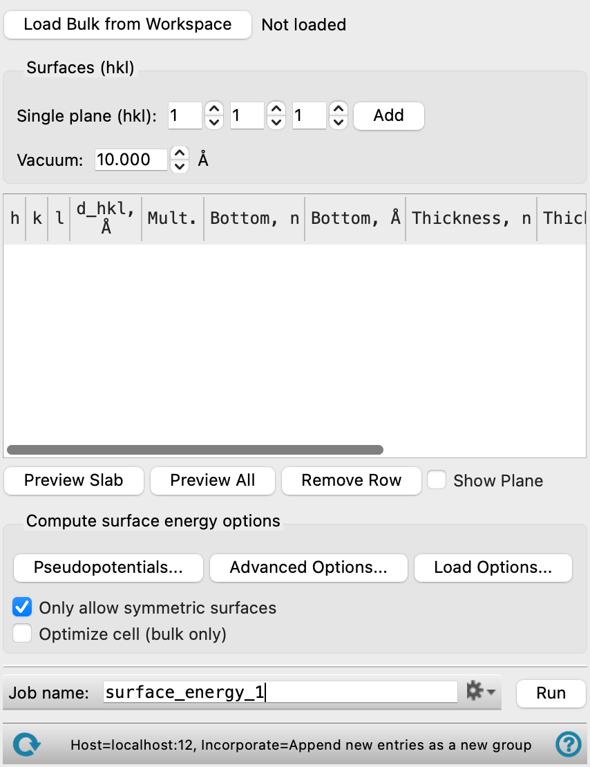
- Load Bulk from Workspace button
-
Load a crystal structure (asymmetric unit) from which you would like to create the slabs.
- Surfaces (hkl) section
-
Use this section to create slabs from the bulk structure by specifying the Miller indices and add it to the slabs table. Multiple slabs can be added. Once the Miller indices are specified, you cannot edit them in the Slabs table. Instead, you must create a new slab in this section to add to the table.
- Single plane (hkl) text boxes and Add button
-
Specify the Miller indices that define the plane used to slice the crystal to generate the slab. Note that the (h k l) plane is relative to the lattice vectors of the input cell, which may be different from the lattice vectors of the conventional unit cell of the crystal. Click the Add button to add it to the Slabs table.
It might be useful to display the planes in the Workspace, on the structure. To do this, you can use the Show Plane option. You might have to extend the crystal to obtain a reasonable view of the planes, which you can also do from the Periodicity toolbox (see Workspace Tools for Periodic Structures).
- Vacuum text box
-
Specify the amount of empty space (measured normal to the surface) to leave above the top surface of the slab in the new periodic system, in angstroms.
- Slabs table
-
Slabs added using the Surfaces (hkl) section are listed here. These settings define the details of the slab and the space above the surface (if any) that defines the new structure. You can use the line to the right of the column header to adjust the width of the columns.
-
h, k, l—The Miller indices as specified in the Single plane (hkl) text boxes when the slab was added. Noneditable.
-
d_hkl— The interplanar distance dhkl, in angstroms. Noneditable.
-
Mult.—The multiplicity of the system. Noneditable.
-
Bottom—Specify the distance along the normal to the chosen plane (defined by the Miller indices) at which the bottom surface of the slab starts, given in terms of the number of cells (n) in the Bottom, n column. The distance is taken normal to the plane. The Bottom, Å column displays the corresponding distance in angstroms. You can use this option to minimize the bonds broken by the the plane used to slice the crystal.
-
Thickness—Specify the thickness of the slab, in terms of the number of cells in the Thickness, n, measured along the c vector. The distance is taken normal to the slab bottom plane. The corresponding thickness in angstroms is displayed in the Thickness, Å column.
-
Vacuum, Å—Specify the amount of empty space (measured normal to the surface) to leave above the top surface of the slab in the new periodic system, in angstroms. The default value is the one used in the Surfaces (hkl) section when you added the slab, but you can adjust the value in the table as well.
-
Fixed atoms—Set Cartesian coordinate constraints on selected atoms, so that the atoms remain at the current values of the constrained coordinates. Click on the Select button to choose atoms to constrain using the Atom Selection Dialog Box. Cannot be used if the Optimize cell (bulk only) option is selected.
-
- Preview Slab button
-
Display the slab corresponding to the selected row in the Workspace. This generates a new entry in Entry List.
- Preview All button
-
Display all slabs listed in the Slabs table in the Workspace. Each unique row generates an entry in the Entry list.
- Remove Row button
-
Remove the selected row from the Slabs table.
- Show Plane option
-
Display the (h k l) plane specified for the slab in the Workspace.
- Compute surface energy options section
-
Run the surface energy calculations using periodic boundary conditions, with Quantum Espresso. You can make settings for the QE calculations using the buttons below.
- Pseudopotentials button
-
Select pseudopotentials for use in the calculations. Opens the Quantum ESPRESSO Calculations - Pseudopotentials Dialog Box. The set of recommended PBE ultrasoft pseudopotentials is distributed with the suite and available from the dialog box. See Installing and Configuring Quantum ESPRESSO for instructions on downloading other pseudopotential sets.
- Advanced Options button
-
Set options for the calculation: spin treatment, density functional, dispersion corrections, Brillouin zone partitioning, occupation, SCF and optimization accuracy
- Load Options button
-
Load option settings from a Quantum ESPRESSO config file (
.cfg). Opens a file selector so you can navigate to and select the config file. The settings replace those in the Quantum ESPRESSO Calculations - Advanced Options Dialog Box. - Only allow symmetric surfaces option
-
Select this option to restrict the surface energy calculations to symmetric surfaces. A warning appears if any slabs are asymmetric.
- Optimize cell (bulk only) option
-
Optimize the cell parameters and atomic coordinates of the bulk unit cell, which is then used to generate slabs. Not compatible with use of hybrid functionals. Cannot be used if the Fixed atoms settings are used.
- Job toolbar
-
Manage job submission and settings. See Job Toolbar for a description of this toolbar.
The Job Settings button opens the Surface Energy Calculations - Job Settings Dialog Box, where you can make settings for running the job.
- Status bar
-
 to reset the panel to its default settings and clear any data from the panel.
If you can submit a job from the panel, the status bar displays information about the current job settings and status for the panel. The settings include the job name, task name and task settings (if any), number of subjobs (if any) and the host name and job incorporation setting. The job status can include messages about job start, job completion and incorporation.
The status bar also contains the Help button
 , which opens an option menu with choices to open the help topic for the panel (Documentation), launch Maestro Assistant, or if available, choose from an option menu of Tutorials. If the panel is used by one or more tutorials, hover over the Tutorials option to display a list of tutorials. Choosing a tutorial opens the tutorial topic.