Quantum ESPRESSO Calculations Panel
Run a periodic DFT calculation with the Quantum Espresso package.
To open this panel, click the Tasks button and browse to Materials → Quantum Mechanics → Quantum ESPRESSO → Quantum ESPRESSO Calculations.
The following licenses are required to use this panel: MS Maestro, Quantum Espresso Interface
- Using
- Features
- Additional Resources
Using the Quantum ESPRESSO Calculations Panel
You must install and configure the Quantum Espresso package to run jobs with this panel—see Installing and Configuring Quantum ESPRESSO for more information. The Quantum ESPRESSO binary version provided as a download (see Installing and Configuring Quantum ESPRESSO) is compiled with OpenMPI for parallelization.
The structures that you choose must contain data for the periodic boundary conditions and include all atoms in the cell (not just the asymmetric unit). The periodic boundary data can be included in PDB style or in Desmond style.
You can run calculations on multiple structures in a single run. The calculation for each structure is run as a subjob, and you can choose the number of subjobs in the Job Settings Dialog Box. If Quantum ESPRESSO was compiled with OpenMP or with OpenMPI, the subjobs themselves can be run in parallel, on a single node (OpenMP and OpenMPI) or multiple nodes (OpenMPI only). The number of threads (also meaning MPI processes) per subjob can be set in the Job Settings Dialog Box.
You can parallelize a subjob over k-points by specifying the number of k-point pools (-npools) in the QE parallel options text box of the Job Settings Dialog Box. The total number of processors must be a multiple of the number of pools: so for example if you choose 4 processors and 2 pools, each pool has 2 processors that it uses to run each k-point in the pool. It does not matter if the number of k-points does not divide evenly into the number of k-point pools: this just results in pools of different sizes.
You can further partition each pool into groups of Kohn-Sham orbitals, or bands, by specifying the number of band groups (-nband) in the QE parallel options text box of the Job Settings Dialog Box. This is especially useful for calculations with hybrid functionals. The total number of processors must be a multiple of the product of the number of bands and number of pools.
In order to allow good parallelization of the 3D FFT when the number of processors exceeds the number of FFT planes, FFTs on Kohn-Sham orbitals can be redistributed to task groups so that each group can process several orbitals at the same time. This is done by specifying the number of task groups (-ntg) in the QE parallel options text box of the Job Settings Dialog Box, and can be done in conjunction with -npools. This is an alternative to using band groups, i.e. (-nband and -ntg are incompatible. It is generally recommended over use of band groups.
This panel contains the basic choices for a 3D periodic DFT calculation with default settings. Settings for control of the calculations can be made in the Quantum ESPRESSO Calculations - Advanced Options Dialog Box. For 2D periodic DFT calculations on a slab, you can use the Effective Screening Medium Calculations Panel.
If you want to use features that are not available in the panels, you can do so from the command line. See Running Quantum ESPRESSO from the Command Line for information.
To write out the input file and a script for running the job from the command line, click the arrow next to the Settings button  and choose Write.
To open a results or viewer panel from the entry group for the results of a Quantum ESPRESSO job . The items on the menu depend on the properties generated by the job.
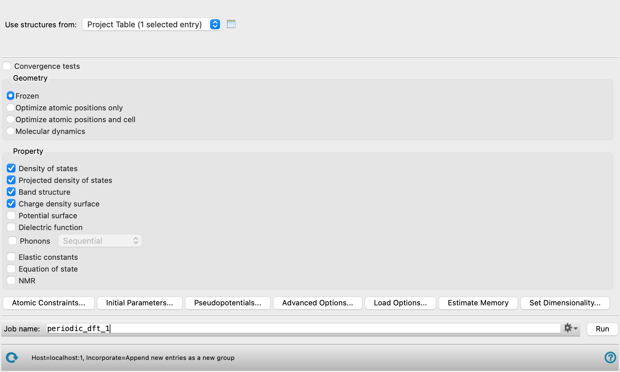
Quantum ESPRESSO Calculations Panel Features
- Use structures from option menu
- Open Project Table button
- File name text box and Browse button
- Convergence tests option
- Geometry section
- Property section
- Atomic Constraints button
- Initial Parameters button
- Pseudopotentials button
- Advanced Options button
- Load Options button
- Estimate Memory button
- Set Dimensionality button
- Job toolbar
- Status bar
- Use structures from option menu
-
Choose the structure source for the periodic DFT calculation. The structures must have data for the periodic boundaries, and all atoms in the cell must be present, not just the asymmetric unit.
- Project Table (n selected entries)—Use the entries that are currently selected in the Project Table or Entry List. The number of entries selected is shown on the menu item.
- Workspace (n included entries)—Use the entries that are currently included in the Workspace, treated as separate structures. The number of entries in the Workspace is shown on the menu item.
- File—Use the specified file. When this option is selected, the File name text box and Browse button are displayed.
- Project Table (n selected entries)—Use the entries that are currently selected in the Project Table or Entry List. The number of entries selected is shown on the menu item.
- Open Project Table button
-
Open the Project Table panel, so you can

- File name text box and Browse button
-
Enter the file name in this text box, or click Browse and navigate to the file. The name of the file you selected is displayed in the text box.
- Convergence tests option
-
Select this option to run convergence tests on the energy threshold and k-point mesh.
- Geometry section
-
Select an option for optimization of the geometry.
-
Frozen—Do not optimize the geometry at all.
-
Optimize atomic positions only—Optimize only the positions of the atoms, with the unit cell held fixed. To optimize atomic positions with a hybrid functional and a pseudopotential, you can only use a norm-conserving (NC) pseudopotential.
-
Optimize atomic positions and cell—Optimize the positions of the atoms and the unit cell parameters, with a target pressure. No constraints are applied to the cell parameters. Not compatible with use of hybrid functionals.
-
Molecular dynamics—Run a Born-Oppenheimer molecular dynamics calculation, with the unit cell held fixed. The trajectory is imported into the project when the job finishes, and can be viewed in the Trajectory Player. To do this, click the T button for the project entry in the Entry List or the Project Table.
-
- Property section
-
Select options for the calculation of properties:
-
Density of states—generate density of states information. When the job has finished, you can create a plot in the Density of States Viewer Panel.
-
Projected density of states—generate projected density of states information, projected to atoms and atomic orbitals. When the job has finished, you can create plots in the Projected Density of States Viewer Panel. The atomic Lowdin charges and derived partial charges, Lowdin spilling parameter, and spin-up and spin-down populations are added as atom-level properties to the output structure. The Lowdin atomic partial charges can be used for MD simulations, as these charges are set as the force-field custom charges (
r_ffio_custom_charge). -
Band structure—generate band structure information. When the job has finished, you can create a plot in the Band Structure Viewer Panel.
-
Charge density surface—generate charge density and spin density on a grid that can be used for plotting. The total (valence) charge density and the difference between this density and the sum of atomic densities are generated. If the system is spin-polarized, the spin-up, spin-down, and polarization (spin-up minus spin-down) densities are also generated. These surfaces can be viewed in Maestro via the Surface Manager Panel. The charge density surface is calculated in the first unit cell. If the structure is not in the first unit cell, the charge density surface may not be aligned with the structure. Use the Translate to First Unit Cell button from the Workspace Tools for Periodic Structures to translate the atoms of the structure into the first unit cell.
-
Potential surface—generate a potential surface on a grid that can be used for plotting. The surface is the sum of the local ionic (bare) and Hartree potentials. These surfaces can be viewed in Maestro via the Surface Manager Panel.
-
Dielectric function—calculate the dielectric function ε. The calculations must be run with norm-conserving pseudopotentials, and the wave function cutoff should be increased to about 60 Ry and the charge density cutoff to about 4 times this value (240 Ry). These settings can be made in the Advanced Options Dialog Box, SCF tab. You can also set the broadening to be used in the Quantum ESPRESSO Calculations - Advanced Options Dialog Box, in the Dielectric function tab. Calculation of the dielectric function requires fixed occupations. The results can be viewed in the Dielectric Function Viewer Panel.
-
Phonons—calculate phonon band dispersion and density of states using density functional perturbation theory (DFPT). Choose between Sequential, Distributed, and Finite difference for job submission for the phonon calculation. For Distributed, a separate job is submitted for each irreducible representation. In the case of fixed occupations, the dielectric constant and IR spectrum are computed. When the job has finished you can plot the phonon density of states as a function of frequency and display the tensors for the dielectric constant (only for fixed occupations) in the Phonon Density of States Viewer Panel, plot the IR spectrum in the Spectrum Plot Panel (only for fixed occupations), or view the normal modes in the Workspace using the Vibrations Panel. For Γ-point only calculations with a Monkhorst-Pack of 1 x 1 x 1, the phonon density of states and band dispersion are not calculated.
-
Elastic constants—calculate elastic constants from the stress tensor, which is obtained from separate calculations done with 24 finite deformations of the cell in which the atomic positions are optimized with the strained cell. Three Maestro properties are returned: Young's Modulus (MPa), Universal Anisotropy, and Poisson Ratio. The input structure must be a fully relaxed cell, which you can request with the Optimize atomic positions and cell option in the Geometry section, if the cell is not already fully relaxed. You can view the results in the Elastic Constants Results Viewer Panel.
-
Equation of state—calculate the energy-volume equation of state from a set of isotropic deformations of the system. You can view the results in the Equation of State Viewer Panel.
-
NMR—calculate the magnetic susceptibilities and NMR chemical shifts for all atoms with the gauge including projector augmented waves method (GIPAW). You need to select a suitable pseudopotential for NMR calculations in the Pseudopotentials Dialog Box such as the GIPAW pseudopotentials by Davide Ceresoli. You can adjust the displacement wave-vector in the Advanced Options Dialog Box, NMR tab. You can view the results in the NMR Viewer Panel.
Note that properties cannot be calculated with hybrid functionals, except for the density of states and projected density of states.
-
- Atomic Constraints button
-
Set or remove Cartesian constraints for atoms in the system. Opens the Atomic Constraints Dialog Box, where you can choose the constraint type (X, Y, Z, or all three), and pick atoms in the Workspace or use the Workspace selection to apply the constraints to. You can delete selected or all constraints.
- Initial Parameters button
-
Set the initial magnetization (
starting_magnetization) value and Hubbard U (Hubbard_U) and J0 (Hubbard_J0) parameters for atoms in the system. Opens the Initial Parameters dialog box, where you can pick atoms in the Workspace and set the values. The initial magnetization for a specified atom can take values between −1 (all spins down) and +1 (all spins up); the value applies to the valence electrons of the atom or ion. Alternatively, you can set the spin values, which is the difference in the number of up and down spin valence electrons (Nα−Nβ), and is proportional to the initial magnetization. The Hubbard U and J0 parameters are only used if you turn on DFT+U calculations in the Quantum ESPRESSO Calculations - Advanced Options Dialog Box. These parameters are given in eV, and can be set for a restricted range of elements, which includes the d and f block elements and C, H, O, N, As, Ga, In.You can delete selected or all settings using the Delete and Delete All buttons.
-
Optionally set the Total magnetization(
tot_magnetization) and Total charge (tot_charge) values for the system. The total magnetization is defined as (majority spin charge − minority spin charge), so 0 represents a singlet, 1 represents a doublet, 2 represents a triplet, and so on. If the value is unspecified, the magnetization is determined during the SCF cycles. If you specify the total magnetization you should not specify initial magnetizations. - Pseudopotentials button
-
Select pseudopotentials for use in the calculations. Opens the Quantum ESPRESSO Calculations - Pseudopotentials Dialog Box. The set of recommended PBE ultrasoft pseudopotentials is distributed with the suite and available from the dialog box. See Installing and Configuring Quantum ESPRESSO for instructions on downloading other pseudopotential sets.
- Advanced Options button
-
Set options for the calculation: spin treatment, density functional, dispersion corrections, Brillouin zone partitioning, occupation, SCF and optimization accuracy
- Load Options button
-
Load option settings from a Quantum ESPRESSO config file (
.cfg). Opens a file selector so you can navigate to and select the config file. The settings replace those in the Quantum ESPRESSO Calculations - Advanced Options Dialog Box. - Estimate Memory button
-
Estimate the memory needed for the selected calculations on the first input structure. After clicking the button, an Info dialog appears with the information. The estimated memory given is for a single CPU. This allows you to assess whether you have sufficient computational resources for a desired calculation without having to first run the calculation.
- Set Dimensionality button
-
Specify whether the system is a slab or bulk material. Opens the Set Dimensionality Dialog Box.
- Job toolbar
-
Manage job submission and settings. See Job Toolbar for a description of this toolbar.
The Job Settings button opens the Quantum ESPRESSO Calculations - Job Settings Dialog Box, where you can make settings for running the job.
- Status bar
-
The status bar displays information about the current job settings and status for the panel. The settings includes the job name, task name and task settings (if any), number of subjobs (if any) and the host name and job incorporation setting. The job status can include messages about job start, job completion and incorporation.
Use the Reset button
 to reset the panel to its default settings and clear any data from the panel.
 The status bar also contains the Help button
 , which opens the help topic for the panel in your browser. If the panel is used by one or more tutorials, hovering over the Help button displays a
  button, which you can click to display a list of tutorials (or you can right-click the Help button instead). Choosing a tutorial opens the tutorial topic.
Tutorials
- NMR Spectra Prediction
- Machine Learning Force Field
- Electronic Structure Calculations of Bulk Crystals Using Quantum ESPRESSO
- Modeling Surfaces
- Calculating Voltage Curves of Spinel Intercalation Compounds
- Ab initio Molecular Dynamics Simulations of Li-ion Diffusion in Solid State Electrolytes
Videos