Trajectory Electrostatic Potential Analysis Panel
Calculate the charge density and the electrostatic potential of a planar interface or micelle from the frames of a trajectory.
To open this panel: click the Tasks button and browse to Materials → Classical Mechanics → Trajectory Analysis → Trajectory Electrostatic Potential Analysis Calculations.
For a tutorial, see Calculating Surfactant Tilt and Electrostatic Potential of a Bilayer System
The following licenses are required to use this panel: MS Maestro
- Overview
- Using
- Features
- Additional Resources
Overview of Trajectory Electrostatic Potential Analysis
The Trajectory Electrostatic Potential Analysis panel allows you to calculate the charge density and electrostatic potential of systems such as bilayers, inorganic interfaces, and surfactant micelles. You can use the charge density to analyze the distribution of charges in the system and the electrostatic potential to measure the work needed to move a charged particle in the system.
For micellar systems, the electrostatic potential ϕ is calculated as a function of the radial distance from a reference point, around which the trajectory is centered. This reference (r=0) is defined as the center of the micelle, and the electrostatic potential is calculated by radial integration of the electric field:

The radial electric field E(r) is defined as:

where ϵs is the relative permittivity of the solvent, ϵ0 is the vacuum permittivity, and ρ is the charge density. It is important to note that the charge density is calculated using the formal charge on individual atoms. Any atom with a formal charge of 0 is ignored. The electrostatic potential is set to zero at radial distances far from the micelle center.
For planar interfaces perpendicular to the z-direction, the trajectory is divided into bins of a user-specified thickness along the xy-plane. The average ion distribution from each bin is used to obtain the charge density, which is then integrated along the z-direction for the electrostatic potential. The reference is the xy-plane in the middle of the solvent region. The calculation of the electrostatic potential ϕ is can be written as:

where zm is the z value of the reference plane. The electrostatic potential is set to zero for the reference plane.
Using the Trajectory Electrostatic Potential Analysis Panel
The input to this panel is the trajectory from an MD simulation. The analysis works best for simulations with constant volume, i.e. run in the NVT ensemble. Although it is possible to use a simulation in the NPT ensemble, the lack of constant volume presents difficulties in averaging over the trajectory and hence can result in artifacts in the density at the edges of the simulation box if the volume fluctuation is not very small. The system should be well equilibrated.
For systems with planar interfaces, interfaces need to be perfectly perpendicular to either the x-, y-, or z-axis. For micellar systems, inputs should be limited to systems containing 1 micelle only. You can build both planar interfaces and micelles using the Build Structured Liquid Panel
To visualize the results, you can use the Trajectory Electrostatic Potential Analysis Viewer Panel (Click the Tasks button and browse to Materials → Classical Mechanics → Trajectory Analysis → Trajectory Electrostatic Potential Analysis Results).To open this panel from the entry group for the results of a job .
.
To write out the input file and a script for running the job from the command line, click the arrow next to the Settings button  and choose Write.
Trajectory Electrostatic Potential Analysis Panel Features
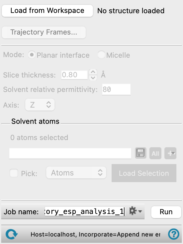
- Load from Workspace button
-
Load the trajectory associated with the structure in the Workspace. The title of the Workspace structure is shown next to this button when the trajectory has been loaded.
- Trajectory Frames button
-
Set the range and interval of trajectory frames to use in the analysis. The total number of frames to be used and the time range (in ns) corresponding to the selected frames are shown to the right of the button. Opens the Trajectory Frames dialog box, in which you can set the following:
-
- Frame range text boxes—Set the range of frames to use. You can also use the slider to select the range.
- Step size text box—Set the interval at which trajectory frames are taken. For a step size of n, every nth frame is taken within the selected range. The first and last frames are always included. Increasing the step size decreases the number of frames to be used and the computational time needed.
- Frames text—Lists the corresponding frame numbers of the selected frame range and step size.
- Time text—Lists the corresponding time range and interval (in ns) of the selected frame range and step size.
- OK button—Apply the selected trajectory frame range and step size and close the dialog box.
- Mode options
-
Select the type of system for which you wish to calculate the trajectory electrostatic potential. See Overview of Trajectory Electrostatic Potential Analysis.
- Planar interface
-
Select this option if the system is a planar interface such as a bilayer. The trajectory is centered on plane in the middle of the solvent region parallel to the interface.
- Micelle
-
Select this option if the system is a micelle. The analysis can only be performed on systems containing a single micelle. The trajectory is centered on the middle of the micelle.
- Slice thickness text box
-
Set the slice thickness for binning the trajectory, in angstroms. This option allows you to choose an approximate slice thickness. The thickness you supply is adjusted to the nearest value that results in an integer number of bins in the box for a planar interface, or spherical shells for a micelle. The slice thickness determines the resolution of the plot lines in the Trajectory Electrostatic Potential Analysis Viewer Panel.
- Solvent relative permittivity text box
-
Set the relative permittivity for the solvent (εs). The default value (80) is for water.
- Axis option menu
-
Select the axis that runs perpendicular to the planar interface. Only present if Planar interface is chosen as the mode.
- Solvent atoms section
-
Select the atoms or molecules in the solvent region. The average plane calculated from the selection is used as the reference plane on which the trajectory is centered. If there is a mixture of solvents that are homogeneously distributed in the solvent region, you can select just one solvent. This section contains a standard set of picking tools that you can use to select a group of atoms. Only present if Planar interface is chosen as the Mode.
- Micelle species option menu
-
Select only the molecules that make up the micelle. The average position of the selection is used as the reference point on which the trajectory is centered. Only present if Micelle is chosen as the mode.
- Job toolbar
-
Manage job submission and settings. See Job Toolbar for a description of this toolbar.
The Job Settings button opens the Trajectory Electrostatic Potential Analysis - Job Settings Dialog Box, where you can make settings for running the job.
- Status bar
-
 to reset the panel to its default settings and clear any data from the panel.
If you can submit a job from the panel, the status bar displays information about the current job settings and status for the panel. The settings include the job name, task name and task settings (if any), number of subjobs (if any) and the host name and job incorporation setting. The job status can include messages about job start, job completion and incorporation.
The status bar also contains the Help button
 , which opens an option menu with choices to open the help topic for the panel (Documentation), launch Maestro Assistant, or if available, choose from an option menu of Tutorials. If the panel is used by one or more tutorials, hover over the Tutorials option to display a list of tutorials. Choosing a tutorial opens the tutorial topic.