Solvation Builder Panel
Build a large solvated system around solutes or on a substrate. The resulting structure can be prepared for molecular dynamics simulations.
To open this panel, click the Tasks button and browse to Materials → Structure Builders → Solvate System.
The following licenses are required to use this panel: MS Maestro, OPLS (optional), MS Force Field Applications (optional)
- Using
- Features
- Additional Resources
Using the Solvation Builder Panel
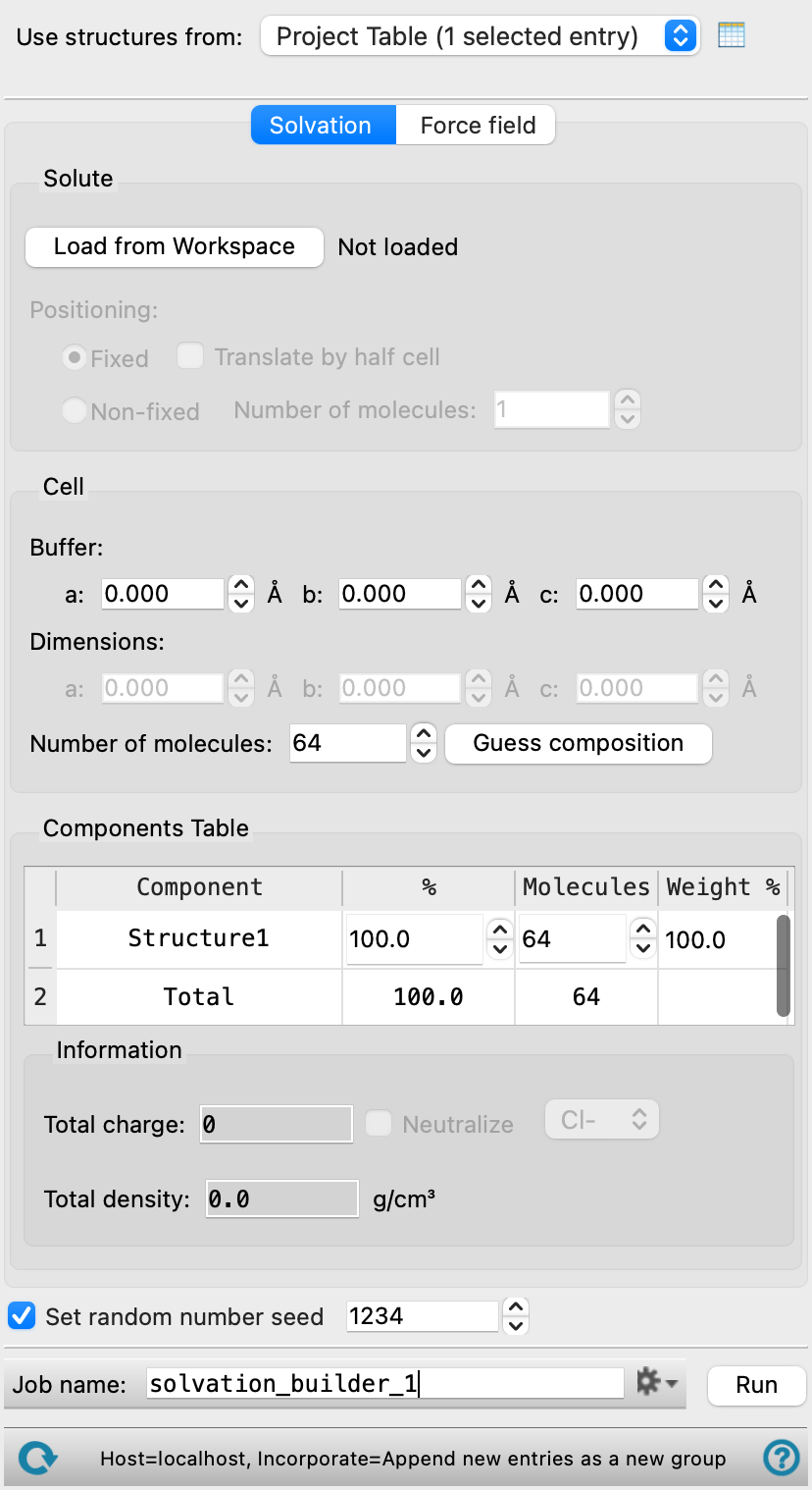
This panel is used to build an orthorhombic cell that contains a large solvated system. The building is done with the PackMol program. This allows you to build structures containing more than 100 thousand atoms in all-atom systems and millions of particles in coarse-grained systems in a reasonable amount of time. You can place solvents around solute molecules distributed in the cell, or on a substrate.
By default, the output consists of Maestro files that contain any periodic boundary condition properties. The file containing the solvated system is named jobname-out.maegz, so you should choose a descriptive job name (rather than the default). Maestro files containing structures for each component (solute/substrate and solvent) are named component_name_n.maegz, where n is the component number in the Components table. Systems with less than 2,000,000 atoms (for all-atom systems) or particles (for coarse-grained systems) built using this panel are automatically incorporated in the workspace. For systems any larger, the output solvated system is written to the job directory, but it is not incorporated.
If you select the option to assign the force field in the Force field tab, the panel prepares a Desmond system. The output includes a CMS (.cms) file, named jobname-out.cms, which you can use directly in Desmond MD simulations. Once you have built a model system, you may want to use the Prepare for MD Panel to prepare for further simulations or equilibrate it or run a series of MD steps with the MD Multistage Workflow Panel. To open this panel from the entry group for the results of a job .
.
To write out the input file and a script for running the job from the command line, click the arrow next to the Settings button  and choose Write.
Please cite the PackMol references [27, 28] in any publication that contains results from the use of this panel.
Solvation Builder Panel Features
- Use structures from option menu
-
Choose the structure source for the solvents.
- Project Table (n selected entries)—Use the entries that are currently selected in the Project Table or Entry List. The number of entries selected is shown on the menu item.
- File—Use the specified file. When this option is selected, the File name text box and Browse button are displayed.
- Project Table (n selected entries)—Use the entries that are currently selected in the Project Table or Entry List. The number of entries selected is shown on the menu item.
- Open Project Table button
-
Open the Project Table panel, so you can

- File name text box and Browse button
-
Enter the file name in this text box, or click Browse and navigate to the file. The name of the file you selected is displayed in the text box.
- Solvation tab
-
Define the components and set solvation parameters for the system.
- Solute section
-
Define the structures around which solvent molecules are placed. This may be solute molecules or a substrate.
- Load from Workspace button
-
Use the structure included in the Workspace for the solute. If you change the included structure in the Workspace, you must press the Load from Workspace button to update the panel. You can load both periodic and non-periodic systems. If you want to load multiple distinct solutes, you must place them in a single entry.
- Positioning options
-
- Fixed and Translate by half cell options
-
If the system imported in the Solute section is periodic, the position of the structure is held fixed while solvent molecules are packed around it. You can control how the solvents are incorporated using the Cell buffer text boxes. For example, if a substrate is loaded as the Solute and you would like to place solvents on top in one direction, you can increase the Cell buffer in only that direction.
The PackMol program requires that all atoms in the system are within the first cell, that is, all the fractional coordinates are within the range (0,1). If instead the solute is centered around the origin and the fractional coordinates are within the range (-0.5, 0.5), the cells needs to be translated by selecting Translate by half cell option so that all coordinates are inside the first cell.
Not available for non-periodic systems.
- Non-fixed option and Number of molecules text box
-
If the system imported in the Solute section is non-periodic, this option is automatically selected. Specify how many molecules of the solute should be in the system with the Number of molecules text box. The molecules are randomly distributed in the cell, but in the same conformation as the initial structure.
Not available for periodic systems.
- Cell section
-
Define the cell size for the simulation box.
- Buffer text boxes
-
If the system imported in the Solute section is periodic, its cell dimensions are imported in the Dimensions text boxes. You can use the Buffer text boxes to increase the cell length along the a, b, and c dimensions in angstroms. The values specified in the Buffer text boxes are automatically added to the dimensions. Use the Total density text box to ensure that the cell is not over-packed.
If the system imported in the Solute section is non-periodic, the values in the Buffer text boxes are not used and Dimensions should be used to specify the cell size instead.
- Dimensions text boxes
-
Set the a, b, and c cell lengths (in angstroms) for the resultant orthorhombic system. You must set the cell dimensions manually if the system imported in the Solute section is non-periodic. You can use the Total density text box to ensure that the cell is not over-packed.
If the system imported in the Solute section is periodic, the Dimensions text box is populated with the dimensions of the system and is noneditable. You must use the Buffer text boxes to adjust the cell size.
Cells should have a total length of 10 Å along each dimension.
- Number of molecules text box
-
Enter the total number of solvent structures to include in the simulation box.
- Guess composition button
-
Click this button to change the number of solvent molecules to target a total density of 1 g cm-3 for the cell, with an equal weight distribution for each solvent in the Components table. If the total density is greater than one and cannot be decreased using this button, increase the Cell buffer or Cell dimensions and try again. This feature may not perform well for large solvents.
- Components Table
-
The table in the Solvation tab lists the solvent components that you selected for inclusion in the simulation box. It is updated whenever you choose a structure source. The percentages (by number) are initially set to be equal. You can edit the table cells to change the composition. As you edit the cells, the values in the unedited percentage cells are adjusted so that the values add up to 100. Once you have edited all cells, you can change any of the values, but the other values are no longer adjusted.
The percentages are used to determine the number of structures of each type, by multiplying them by the total number of structures, and dividing by 100, then rounding up to the nearest integer. The percentages or proportions you provide will therefore not be exact, and must be regarded as a target value. However, you must ensure that the number of structures for each component, which is reported in the Molecules column, adds up to the total. If it does not, you must adjust either the percentages or the number of structures, by editing either the percentage column or the Molecules column.
For example, if you have an odd number of structures in a two-component mixture, the default percentages are both 50, and the number of structures does not add up to the total, as both are rounded up. You must change one of the components to have one more structure than the other.
The percentage by weight of the components is reported in the Weight % column. You cannot adjust this value directly; it is computed from the values in the other columns and the molecular weights of the components. The Weight % column is not present for coarse-grained systems.
- Information section
-
- Total charge text box
-
Displays the total charge for the system. The charge value automatically updates when the settings in the panel are changed. Noneditable.
- Neutralize option and option menu
-
Choose to neutralize the net charge of the system automatically by adding ions. You can choose the ion type from the option menu.
-
This option is helpful as it is usually desirable to have an electrically neutral system for simulation (though not strictly necessary).
- Total density text box
-
Displays the total density as calculated from the settings in the panel. The density value automatically updates when the settings are changed. This value can be used to check that the cell is not over-packed.
Noneditable.
- Use constant radius option and text box
-
Select this option to specify a constant value for radii of particles for faster packing. Only present for coarse-grained systems.
- Set random number seed option and text box
-
Select this option to specify a random seed to be used in building the system. Specifying the seed allows you to reproduce the results, unless other factors affect them. If this option is not selected, a seed is chosen at random.
- Force field tab
-
- Assign force field option and section
-
Select this option to create a Desmond model system (CMS file) for MD simulation as part of the output. The model system requires the specification of the force field. The tools available for specifying the force field depend on whether you have an all-atom or a coarse-grained system.
For all-atom systems, the following tools are available:
- Force Field button
-
Click the Force Field button to specify the force field to use and any custom charges, in the Force Field Dialog Box. The current force field is shown to the left of the button.
- Water model option menu
-
If water is one of the components of the system, choose the water model for the simulations. The water models available on the menu depend on the force field. For OPLS4, the models are SPC, SPCE, TIP3P, TIP4P, TIP4P2005, TIP4PEW, TIP5P, TIP4PD. For OPLS_2005, only the SPC and TIP3P models are available. If the water model is already assigned, choose Current to retain this model.
-
Only present when the system is an atomistic system.
- Redistribute heavy atom mass to hydrogens option
-
Redistribute some of the mass of heavy atoms to bonded hydrogen atoms. This allows shorter time steps to be used and avoid some of the instability due to high-frequency hydrogen motions.
Only present when the system is an atomistic system.
- Coarse-grained force field option menu
-
Choose the coarse-grained force field for the MD simulations. The choices depend on the Location option selected. The installation contains the Martini and Martini_solution force fields. The menu is populated with the coarse-grained force fields you have saved if you choose Local for the Location.
- Description button
-
Display a description of the chosen force field in a separate panel.
- Location options
-
Select an option for the location of the coarse-grained force field. The force fields listed on the Force field option menu depend on this choice.
- Installation—use the force fields in the installation. These are the Martini, Martini_solvation, or Martini_full force fields [15].
- Local—import a force field from your local user resources directory. These are force fields that you have saved for your own use.
- Use particle mesh Ewald Method option
-
Electrostatic interactions are calculated with the particle mesh Ewald (PME) method when using a Martini force field instead of cutoff parameters. Only available if the system is a coarse-grained system and a Martini force field is selected.
- Scale lattice vectors option
-
Scale the volume of the system to match the nonbonded cutoff distance and reduced density of the force field. Only available if the system is a coarse-grained system and a DPD force field is selected.
For coarse-grained systems, the following tools are available:
Manage job submission and settings. See Job Toolbar for a description of this toolbar.
The Job Settings button opens the Solvation Builder - Job Settings Dialog Box, where you can make settings for running the job.
 to reset the panel to its default settings and clear any data from the panel.
If you can submit a job from the panel, the status bar displays information about the current job settings and status for the panel. The settings include the job name, task name and task settings (if any), number of subjobs (if any) and the host name and job incorporation setting. The job status can include messages about job start, job completion and incorporation.
The status bar also contains the Help button  , which opens an option menu with choices to open the help topic for the panel (Documentation), launch Maestro Assistant, or if available, choose from an option menu of Tutorials. If the panel is used by one or more tutorials, hover over the Tutorials option to display a list of tutorials. Choosing a tutorial opens the tutorial topic.