Trajectory Player
The Trajectory Player enables you to play through trajectories from Desmond simulations and Quantum Espresso MD calculations, examine individual frames, and export trajectory data in a variety of forms.
To display the Trajectory Player, double-click the T button in the Title column of an entry in the Entry List or Project Table, or click this button and choose Load Trajectory.
If the trajectory is missing (i.e. is not in the same directory as the associated CMS file that was imported into Maestro), a dialog box opens, with three actions: locate the trajectory (Import File) and copy it to the directory that the CMS file is in, renaming if necessary; remove the trajectory data from the entry (Remove Data); or cancel the loading of the trajectory (Cancel). If the trajectory has only one frame, the player does not open.
For a tutorial, see Trajectory Plots Guide.
- Using
- Features
- Additional Resources
Using the Trajectory Player
When you open the Trajectory Player, entries in the Workspace that are not fixed are excluded (other than another trajectory entry). You can have a single entry in the Workspace as a reference entry for the trajectory. The reference can be any suitable entry, including the entry for another trajectory. It must be included and fixed before you include the trajectory entry. If there is more than one reference entry in the Workspace, a warning is posted, and you must exclude entries so that there is not more than one reference entry in the Workspace before you can play the trajectory. If you have two trajectory entries in the Workspace, the trajectory that is played is the one for the entry that is not fixed.
You can make measurements within the trajectory, either on the entry for the trajectory or in a trajectory frame when play is stopped. The measurements are updated as you play through the trajectory to give the values for the current frame. This allows you to monitor changes in bond lengths, angles, and dihedrals. The measurements take account of the periodic boundary conditions to display values for measurements that span the boundary. For other trajectory analysis tools, see Simulation Interactions Diagram Panel and Trajectory Frame Clustering Panel.
You can center the trajectory on specific atoms, so that these are always in the center of every frame. The centered trajectory can be exported with the centering applied. Centering the trajectory can also be done when the job is run, with settings in the Desmond — Advanced Options Dialog Box.
Trajectory Player Features
The trajectory player is a toolbar, with three sections: play controls, frame controls, and buttons for other functions.

Play Controls
The toolbar contains a standard set of controls for playing through the trajectory frames, which are described below.

|
Jump to start
Jump to the first frame. This button replaces the Step back button when playback starts. |

|
Step back (Keyboard shortcut: left arrow when player is paused) Step back to the previous displayed frame. If the step size is set to a value greater than 1 (say M), the frame displayed is the Mth frame backward in the trajectory from the current frame. |

|
Play
Play through the frames in the indicated direction. The direction of play is set in the Playback Settings Pane; the button updates when you switch direction. When you click this button, it is replaced with the Pause button. When playback stops, clicking this button starts playback again from the starting frame (at whichever end is appropriate for the play direction). |

|
Pause
Stop playing through the frames. When you click this button, it is replaced with the Play button. |

|
Step forward (Keyboard shortcut: right arrow when player is paused) Step forward to the next frame to be displayed. If the step size is set to a value greater than 1 (say M), the frame displayed is the Mth frame forward in the trajectory from the current frame. |

|
Jump to end
Jump to the last frame. This button replaces the Step forward button when playback starts. |
Frame controls
This section has controls for the display of individual frames and for playing through the frames.
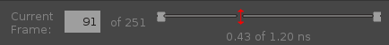
- Current Frame text box
-
This text box displays the current frame number. Frames are numbered from 1. Play starts from this frame. The total number of frames is reported to the right.
You can edit the frame number to change the current frame. The current frame marker on the slider moves to mark the new current frame. If you click in the text box during playback, playback pauses until you move the pointer out of the text box, when playback resumes.
- Frame slider
-
The slider marks the starting and ending points of trajectory playback, and the current frame. You can drag the two markers at the ends to set the start and end frame to be used in playback. You can also the current frame marker to a new location (which updates the frame number in the Current Frame text box). If you try to drag the start or end marker past the current frame marker, the current frame marker is dragged along as well. A tooltip for each marker displays the frame number and time, and is displayed while you drag the marker.
- Trajectory time display
-
The trajectory time at the current frame and the total trajectory time is shown below the frame slider.
Buttons
- Export button
-

Export individual frames, all frames, or a selection of frames as structures, as an image, or as a movie. Clicking this button opens a menu, from which you can choose the export type:-
Structures—Save structures from the trajectory to a file or create project entries from the structures. Opens the Trajectory Player — Export Structures Dialog Box in which you can specify where the structures will go, which structures to export, and which atoms to export.
-
Trajectory—Export the trajectory and the structure to a new CMS file and trajectory, with a new name. The playback settings made in the trajectory player are applied to the trajectory before export (such as positioning). Opens a file selector so you can navigate to a location and save the CMS file and trajectory.
-
Image—Create an image of the Workspace with the current frame displayed. Opens the Save Image Dialog Box.
-
Movie—Save a movie of the trajectory in MPEG format. Opens the Export Movie Dialog Box, in which you can select the format and the frames to be exported.
There is also an item for displaying multiple frames from a trajectory:
-
View Snapshots—Display multiple frames from a trajectory (snapshots), superimposed in the Workspace, optionally color-coded by simulation time. Opens the Display Trajectory Snapshots Panel. You can export snapshots from this panel.
-
- Playback Settings button
-

This button opens the Playback Settings Pane in which you can make settings to control all aspects of the playback. The current settings in this pane are used for any trajectory for which playback settings have not been explicitly made. This means that you can make settings for one trajectory, then play another trajectory with the same settings. - Plot button
-

Plot properties computed over all trajectory frames as a function of simulation time. First the Compute Properties Over Trajectory menu opens, so you can calculate the properties:- Measurements
-
Plot measurements made between atoms in the Workspace. The choices available on the submenu are:
- Currently in Workspace—plot the measurements that have already been made for the current Workspace structure. The measurements do not need to be displayed to be plotted.
- Add Workspace Measurement—add a measurement to the Workspace structure. Opens the Measurement banner for defining the measurement.
- Planar Angle—plot the angle between two planes. Opens the Planar Angle banner to define the planes. The planar angle is displayed in the Workspace.
- Interaction Counts
-
Plot counts of selected interactions as a function of simulation time. The interactions that are available and the interacting atoms are set up in the Interactions Toolbox. The full range of choices on the submenu is as follows; individual items may be unavailable because of the settings in the Interactions Toolbox.
- All Types—plot counts of all types of interactions
- Hydrogen Bonds—plot hydrogen bond counts
- Halogen Bonds—plot halogen bond counts
- Salt Bridges—plot counts of salt bridges
- Pi-Pi Stacking—plot counts of pi-pi stacking interactions
- Pi-Cation—plot counts of pi-cation interactions
- For Visible Atoms Only—calculate and plot counts for the displayed atoms; if this item is deselected, counts are calculated and plotted for all atoms.
- Descriptors
-
Plot values of descriptors defined for the atoms that are selected in the Workspace. The choices available on the submenu are:
- RMSD—plot the RMS deviation of the selected atoms from those in a reference. By default, the reference is the first frame. You can set the reference in the RMSD Settings dialog box, which you open by choosing View RMSD Settings from this submenu.
- Radius of Gyration—plot the radius of gyration of the selected atoms.
- Polar Surface Area—plot the combined surface area of the polar atoms in the atom selection.
- Solvent Accessible Surface Area—plot the solvent-accessible surface area of the selected atoms.
- Molecular Surface Area—plot the surface area of the atoms in the selection when considered as an entire molecule.
- View RMSD Settings—open the RMSD/RMSF Settings dialog box so you can set up the RMSD measurement. The RMSD can be calculated with respect to a chosen frame (default is frame 1) or a structure in the project or a file; and the atoms used for superposition before the RMSD is calculated can be defined.
- RMSF
-
Plot the time-averaged RMS fluctuations for the atoms that are selected in the Workspace. The RMSF plots are shown in the Advanced Plots section. The choices available on the submenu are:
- Per Atom—plot the RMS fluctuation of the selected atoms from those in a reference. By default, the reference is the first frame. You can set the reference in the RMSD/RMSF Settings dialog box, which you open by choosing View Settings from this submenu.
- Per Residue—plot the RMSF of the selected atoms averaged per residue.
- View Settings—open the RMSD/RMSF Settings dialog box so you can set up the RMSF measurement. The RMSF can be calculated with respect to a chosen frame (default is frame 1) or a structure in the project or a file; and the atoms used for the superposition before the RMSF is calculated can be defined.
- Energy Calculations
-
Plot energy components within and between predefined or custom sets of atoms. The energy components are bond, angle, and dihedral energies (calculated only within a set), and Coulomb and van der Waals energies (calculated within and between sets).
The trajectory must have an associated configuration file (
.cfg); if it is not in the same location as the trajectory, you are prompted to locate it.The submenu allows you to choose the sets and make job settings. There is a restriction to a maximum of 10 sets.
- All Substructure Sets (Grouped)—all substructures that appear at the top level of the Structure Hierarchy (shown in the Entry List / Structure Hierarchy panel), such as Protein, Ligand, Waters, Metals/Ions, Membranes.
- All Substructure Sets (Individual)—all substructures at the next level of the Structure Hierarchy, such as each chain or ligand, and Waters, Metals/Ions, Membranes as groups.
- Custom Substructure Sets—a selection of any of the substructures in the Structure Hierarchy. Opens the Define Custom Substructure Sets dialog box to choose the substructures.
- Custom ASL Sets—sets of atoms defined by atom selection. Opens the Define Custom ASL Sets Dialog Box, to define the sets.
- Job Settings—make host settings for running the job. Opens the Job Settings Dialog Box.
- Phi-Psi Angles(Selected Residues)
-
Generate a Ramachandran plot of the protein dihedrals φ and ψ for selected residues. A maximum of 5 residues can be selected, and individual plots are generated for each residue.
-
Once the plot has been generated, you can right-click on the plot to open a context menu, where you can choose to Save Image, Export as CSV, or Export to Excel.
- Conformation Wheel (Selected Residues)
-
Generate backbone and side chain dihedral angle plots for both nucleic acids and proteins, in degrees, in the form of a conformation wheel.
For nucleic acids, these angles are the alpha, beta, gamma, delta, epsilon, chi, and zeta dihedral angles.
For proteins, these angles are phi, psi, and potentially chi angle rings depending on the residue.
Once the plot has been generated, right-click on the conformation wheel plot to open a context menu, where you can choose to Save Image, Export as CSV, Export to Excel, or Delete the plot.
- RDF (Selected Atoms)
-
Calculate the radial distribution function for the selected atoms. Select how centers should be calculated:
- Individual Atoms—use the atoms as the center.
- Residue Centers of Mass—use the residue center of mass to determine the center of the selected atoms.
- Molecule Centers of Mass—use the molecule center of mass to determine the center of the selected atoms.
When the job has run, you can view the RDF plot in the Advanced Plots section of theTrajectory Player, and export the data (function and integral) to a
.xlsxfile with the Export Results button. In the RDF plot, select Show integral to plot the integral of the radial distribution function on the plot as well as the function itself. The integral is evaluated at the same time as the function, so it is displayed immediately. You can use the integral to infer average coordination numbers.When the integral is displayed, the axis on the right side is used to mark the integral values. The ASL expression is included in the title of the plot. Right-click on the plot to access a context menu, where you can save the plot as an image, export the function as a CSV or to Excel, or export all data as a.datfile. - Other RDF
-
Calculate the radial distribution function for a specific set of particles. A particle can be either an individual atom, or the center of a selection of atoms in molecules or residues. Opens the Plot Radial Distribution Function Panel, where you can make certain selections.
When the job has run, you can view the RDF plot in the Advanced Plots section of theTrajectory Player, and export the data (function and integral) to a
.xlsxfile with the Export Results button. In the RDF plot, select Show integral to plot the integral of the radial distribution function on the plot as well as the function itself. The integral is evaluated at the same time as the function, so it is displayed immediately. You can use the integral to infer average coordination numbers.When the integral is displayed, the axis on the right side is used to mark the integral values. The ASL expression is included in the title of the plot. Right-click on the plot to access a context menu, where you can save the plot as an image, export the function as a CSV or to Excel, or export all data as a.datfile.
When you have chosen a property to plot, the values are calculated and plotted in the Plot Computed Values Over Time panel. If this panel is not open, it opens, docked on the right of the Workspace.
RMSF plots, RDF plots, and energy plots are listed in the Advanced Plots section. Clicking on a plot item opens the plot in a separate window (Review Energy Plots Panel for energy plots).
- λ Sites button
-

This button opens a menu which lists the titratable residues selected from the Protein Constant pH Simulations Panel. The dominant protonation state and its lambda value (in %) for the selected trajectory frame is displayed in parenthesis following the residue label. Click on a residue to highlight it in the Workspace.Only present for trajectories run with the Protein Constant pH Simulations Panel.
Shortcut menu
The Trajectory Player has a shortcut menu, with two items: Close, to close the player, and Help, to display this help topic.